Linear Regression, Part 2
Building an Understanding of Gradient Descent Using Computer Programming
Introduction
Thank you for visiting my blog.
Today’s blog is the second blog in a series I am doing on linear regression. If you are reading this blog, I hope you have a fundamental understanding of what linear regression is and what a linear regression model looks like. If you don’t already know about linear regression, you may want to read this blog: https://data8.science.blog/2020/08/12/linear-regression-part-1/ I wrote and come back later. In the blog referenced above, I talk at a high level about optimizing for parameters like slope and intercept. Well, we are going to talk about how machines minimize error in predictive models. We are going to introduce the idea of a cost function soon. Even though we will be discussing cost functions in the context of linear regression, you will probably realize that this is not the only application. That said, the title of this blog shouldn’t confuse anyone and all should understand that gradient descent is more of an overarching subject for many machine learning problems.
The Cost Function
The first idea that needs to be introduced, as we begin to discuss gradient descent, is the cost function. As you may recall, we wrote out a pretty simple calculus formula that found the optimal slope and intercept for the 2D model in the last blog. If you didn’t read last blog, that’s fine. The main idea is that we started with an error function, or MSE. We then took partial derivatives of that function and applied optimization techniques to search for a minimum. What I didn’t tell you in my blog, and people who didn’t read my blog may or may not know is that there is in fact a name for the function that takes a partial derivate in an error function. We call it the cost function. Here is a common representation of the cost function (for 2-dimensional case):
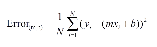
This function should be familiar. This is basically just the sum of model error in linear regression. Model error is what we try to minimize in EVERY machine learning model, so I hope you see why gradient descent is not unique for linear algebra.
What is a Gradient?
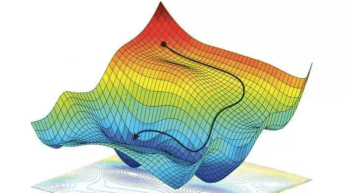
Simply put, a gradient is the slope of a curve, or derivative, at any point on a plane with regards to one variable (in a multivariate function). Since the function being minimized is the loss function, we follow the gradient down (hence the name gradient descent) until it approaches or hits zero (for each variable) in order to have minimal error. In gradient descent, we start by taking big steps and slow down as we get closer to that point of minimal error. That’s what gradient descent is; slowly descending down a curve or graph to the lowest point, which represents minimal error, and finding the parameters that correspond to that low point. Here’s a good visualization for gradient descent (for one variable).
The next equation is one I found online that illustrates how we use the graph above in practice:

The above two visual may seem confusing, so let’s work backwards. W t+1 corresponds to our next predicted value for optimal coefficient value. W t was our previous assumption for optimal coefficient value. The term on the right looks a bit funky, but it’s pretty simple actually. The alpha corresponds to the learning rate and the quotient is the gradient. The learning rate is essentially a parameter that tells us how quickly we move. If it is low, models can be computationally expensive, but if it is high, it may not hit the best concluding point. At this point, we can revisit the gif. The gif shows the movement in error as we iteratively update W t into W t+1.
At this point, I have sort-of discussed the gradient itself and danced around the topic. Now, let’s address it directly using visuals. Now keep in mind, gradients are partial derivatives for variables in the cost function that enable us to search for a minimum value. Also, for the sake of keeping things simple, I will express gradients using the two-dimensional model. Hopefully, the following visual shows a clear progression from the cost function.
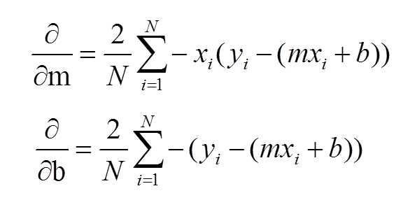
In case the above confuses you, I would not focus on the left side of either the top or bottom equation. Focus on the right side. These formulas should look familiar as they were part of my handwritten notes in my initial linear regression blog. These functions represent the gradients used for slope (m) and intercept (b) in gradient descent.
Let’s review: we want to minimize error and use the derivative of the error function to help that process. Again, this is gradient descent in a simple form:
I’d like to now go through some code in the next steps.
Gradient Descent Code
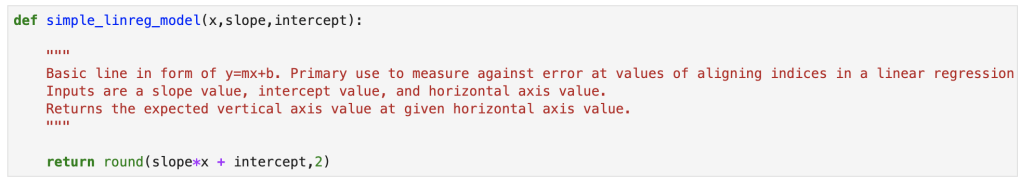
We’ll start with a simple model:
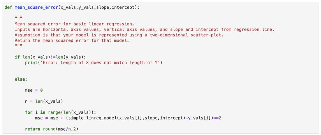
Next, we have our error:
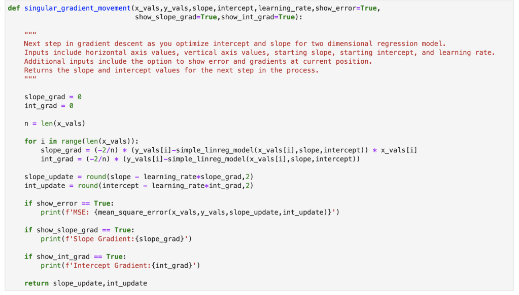
Here we have a single step in gradient descent:
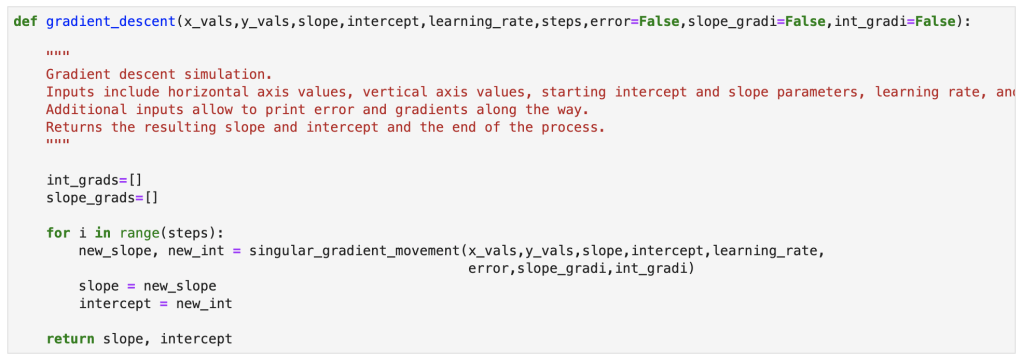
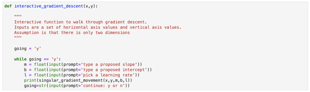
Finally, here is the full gradient descent:
Bonus Content!
I also created an interactive function for gradient descent and will provide a demo. You can copy my notes from this notebook with your own x and y values to run an interactive gradient descent as well.
Demo link: https://www.youtube.com/watch?v=hWqvmmSHg_g&feature=youtu.be
Conclusion
Gradient descent is a simple concept that can be incredibly powerful in many situations. It works well with linear regression, and that’s why I decided to discuss it here. I am told that often times, in the real world, using a simple sklearn or stastsmodels model is not good enough. If it were that easy, I imagine the demand for data scientists with advanced statistical skills would be lower. Instead, I have been told, that custom cost functions have to be carefully though out and gradient descent can be used to optimize those models. I also did my first blog video for today’s blog and hope it went over well. I have one more blog in this series where I go through regression using python.
Sources and Further Reading