Introduction

Often times, when addressing data sets with many features, reducing features and simplifying your data can be helpful. Usually, one particular juncture where you remove a lot of data or features is by reducing correlation using a filter of 70%, or so. (Having highly correlated variables usually leads to overfitting). However, you can continue to reduce features and improve your models by deleting features that not only correlate to each other, but also… don’t really matter. A quick example: Imagine I was trying to predict whether or not someone might get a disease and the information I had was height, age, weight, wingspan, and favorite song. I might have to remove height or wingspan since they probably have a high degree of correlation. Favorite song, on the other hand, likely has no impact on anything one would care about but would not be removed using correlation. That’s why we would just get rid of one feature. Similarly, if there are other features that are irrelevant or can be mathematically proven to have little impact, we could delete them. There are various methods and avenues one could take to accomplish this task. This blog will outline a couple them, particularly: Principal Component Analysis, Recursive Feature Elimination, and Regularization. The ideas, concepts, benefits, and drawbacks will be discussed and some coding snippets will be provided.

Principal Component Analysis (PCA)

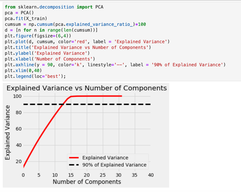
So, just off the bat, PCA is complicated and involves a lot of backend linear algebra and I don’t even understand it fully myself. This is not a blog about linear algebra, it’s a blog about making life easier, so I plan to keep this discussion at a pretty high level. First, I’ll start with a prerequisite; scale your data. Scaling data is a process of reducing impact based on magnitude alone and aligning all your data to be relatively in the same range of values. If you had a data point representing GDP and another data point representing year the country was founded, you can’t compare those variables easily as one is a lot bigger in magnitude than the other. There are various ways to scale your variables and I have a separate blog about that if you would like to learn more. For our purposes, though, we always need to apply standard scaling. Standard scaling takes each unique value of a variable, subtracts its mean, and finally divides by the standard deviation. The effect is that every value becomes compressed to the interval [-1,1]. Next, as discussed above, we filter out correlated variables. Okay, so now things get real. We’re ready to for the hard part. The first important idea to understand beforehand, however, is what a principal component is. Principal components are new features which are some linear representation of operations performed with other features. So If I have the two features weight and height – maybe I could combine the two by dividing weight by height to get some other feature. Unfortunately, however, as we will discuss more later, none of these new components we will replace our features with actually have a name, they are just assigned a numeric representation such as 0 or 1 (or 2 or….). While we don’t maintain feature names, the ultimate goal is to make life easier. So once we have transformed the structure of our features we want to find out how many features we actually need and how many are superfluous. Okay, so we know what a principal component is and what purpose they serve, but how are they constructed in the first place? We know they are derived from our initial features, but we don’t know where they come from. I’ll start by saying this: the amount of principal components created always matches the number of features, but we can easily see with visualization tools which ones we plan to delete. So the short answer to our question of where these things come from is that for each dimension (feature) in our data, we have two corresponding linear algebra metrics/results called eigenvectors and eigenvalues which you may remember from linear algebra. If you don’t, given a square matrix called “A” that has a non-zero determinant; multiplying that matrix by an eigenvector, called v, yields the same result as scaling that vector, v, by a scalar known as the eigenvalue, lambda. The story these metrics tell is apparent when you perform linear transformations. When you transform your axes in transformations, the eigenvectors will still maintain the same direction but will increase in scale by lambda. That may sound confusing, and it’s not critical to understand it completely but I wanted to leave a short explanation for those more familiar with linear algebra. What matters is that calculating these metrics/results in the context of data science gives us information about our features. The eigenvalues with highest magnitude yield the eigenvectors with the most impact on explaining variance in models. Source two below indicates that “Eigenvectors are the set of basis functions that are the most efficient set to describe data variability. The eigenvalues is a measure of the data variance explained by each of the new coordinate axis.” What’s important to keep in mind is that we use the eigenvalues to remind us of what new, unnamed, transformations matter most.

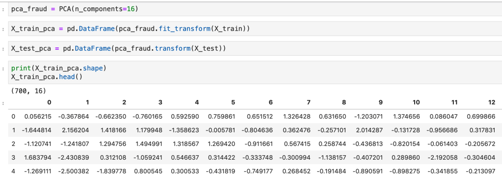
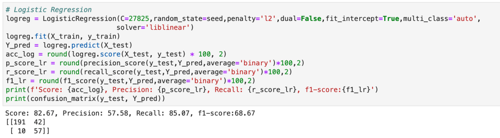
Code (from a fraud detection model)

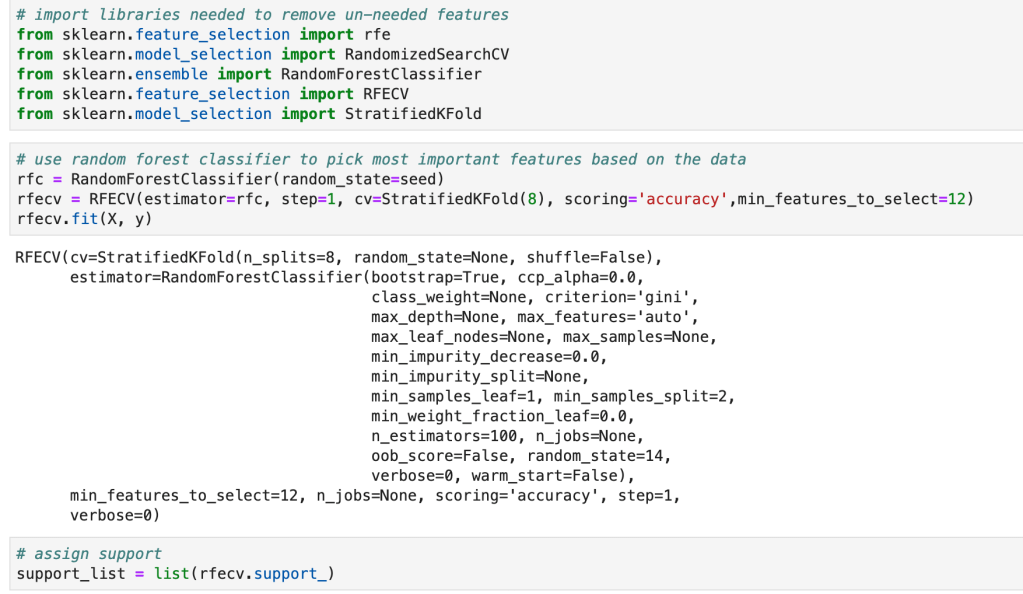
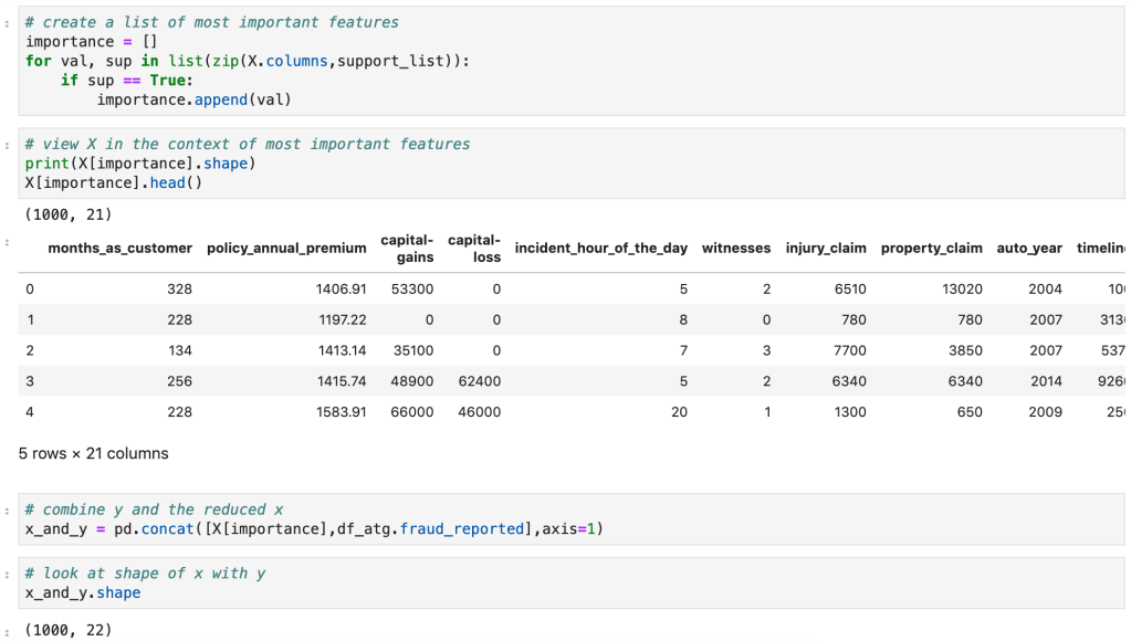
Recursive Feature Elimination (RFE)

RFE is different than PCA in the sense that it models data and then goes back in time so you can run a new model. What I mean by this is that RFE assumes you have model in place and then uses that model to find feature importances or coefficients. If you were running a linear regression model, for example, you would instantiate a linear regression model, run the model, and find the variables with the highest coefficients and drop all the other ones. This can work with a random forest classifier, for example, which has an attribute called feature importances. Usually, I like to find what model works best and then run RFE using that model. RFE will then run through different combinations of keeping different amounts of features and then solve for the features that matter most.

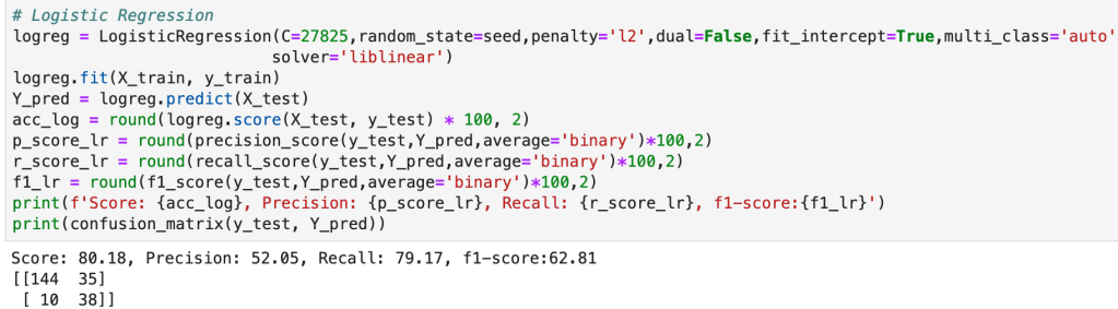
Code

Regularization (Lasso and Ridge)

Regularization is a process designed to reduce overfitting in regression models by penalizing models for having excessive and misleading predictive features. According to Renu Khaldewal (see below): “When a model tries to fit the data pattern as well as noise then the model has a high variance a[n]d will be overfitting… An overfitted model performs well on training data but fails to generalize.” The point is that it works when you train the model but does not deal well with new data. Let’s think back to the “favorite song” feature I proposed earlier. If we were to survey people likely to get a disease and find they all have the same favorite song, while this would certainly be interesting, it would be pretty pointless. The real problem would be when we encounter someone who likes a different song but is checks off every other box. The model might say this person is unlikely to get the disease. Once we get rid of this feature, well now we’re talking and we can focus on the real predictors. So we know what regularization is (a method of placing focus on more predictive features and penalizing models that have excessive features), we know why we need it (overfitting), we don’t yet know how it works. Let’s get started. In gradient descent, one key term you better know is “cost function.” It’s a mildly complex topic, but basically it tells you how much error is in your model by subtracting the predicted values from the true values and summing up the total error. You then use calculus to optimize this cost function to find the inputs that produce the minimal error. Now keep in mind that the cost function captures every variable and the error present in each. In regularization, an extra term is added to that cost function which reduces the impact of larger variables. So the outcome is that you optimize your cost function and find the coefficients of a regression, however you now have reduced overfitting by scaling your terms using a value (often called) lambda and thus have produced more descriptive coefficients. So what is this Ridge and Lasso business? Well, there are two common ways of performing regularization (there is a third, less common, way which basically covers both). In ridge regularization you add a parameter designed to scale the magnitude of each coefficient. We call this L2. Lasso, or L1, is very similar. The difference in effect is that lasso regularization may actually remove features completely. Not just decrease their impact, but actually remove them. So ridge may decrease the impact of “favorite song” while lasso would likely remove it completely. In this sense, I believe lasso more closely resembles PCA and RFE than ridge. In Khandelwal’s summary, she mentions that L1 deals well with outliers but struggles with more complex cases, while ridge has the opposite effect on both accounts. I won’t get in to that third case I alluded above. It’s called Elastic Net and you can use if you’re unsure of whether you want to use ridge or lasso. That’s all I’m going to say… but I will provide code for it.

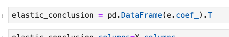
Code

(Quick note: alpha is a parameter which determines how much of a penalty is placed in regression).

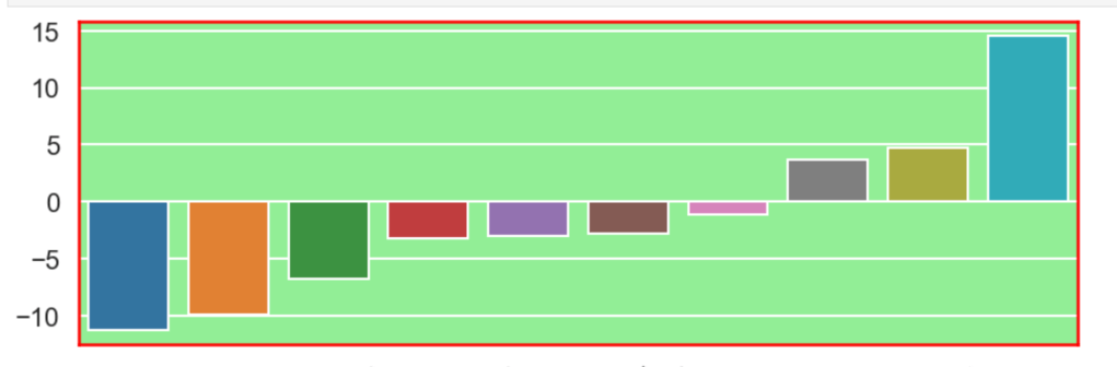
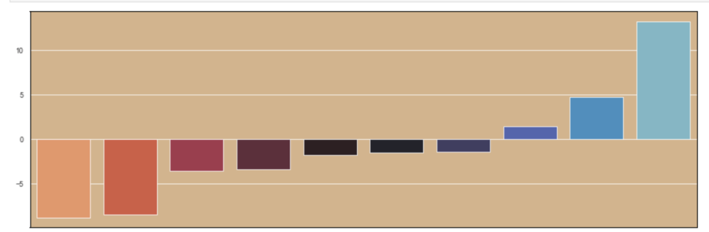
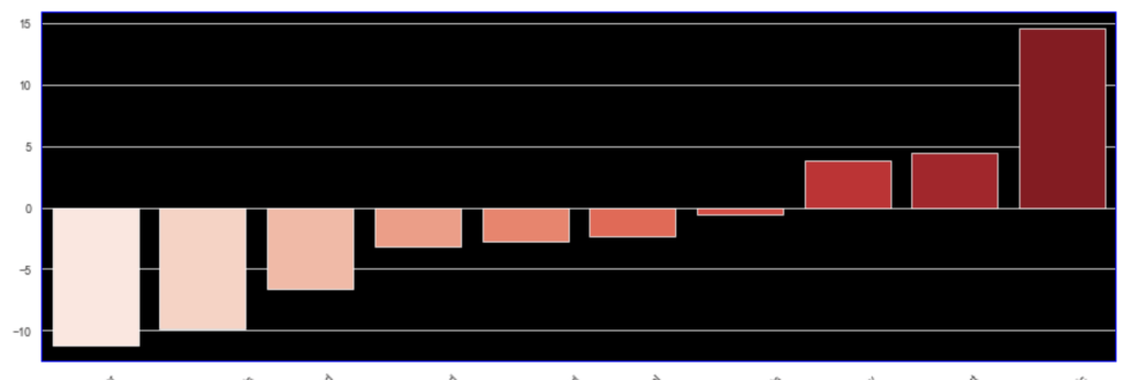
I’ll also quickly add a screenshot to capture context. The variables will not be displayed, but one should instead pay attention to the extreme y (vertical axis) values and see how each type of regularization affects the resulting coefficients.

Initial visual:

Ridge

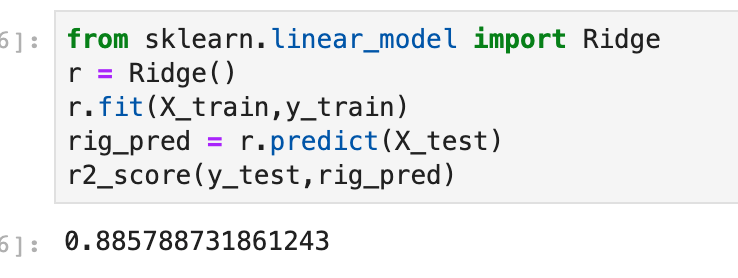
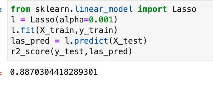
(Quick note this accuracy is up from 86%)

Lasso

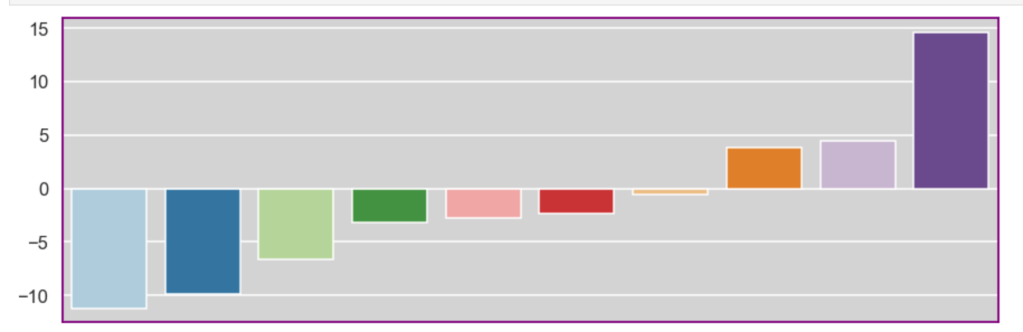
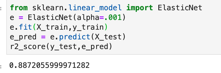
Elastic Net

Conclusion

Data science is by nature a bit messy and inquiries can get out of hand very quickly. By reducing features, you not only make the task at hand easier to deal with and less intimidating, but you tell a more meaningful story. To get back to an earlier example, I really don’t care if everyone whose favorite song is “Sweet Caroline” are likely to be at risk for a certain disease or not. Having that information is not only useless, but it also will make your models worse. Here, I have provided a high-level road map to improving models and distinguishing between important information and superfluous information. My advice to any reader is to get in the habit of reducing features and honing on what matters right away. As an added bonus, you’ll probably get to make some fun visuals, if you enjoy that sort of thing. I personally spent some time designing a robust function that can handle RFE pretty well in many situations. While I don’t have it posted here, it is likely all over my GitHub. It’s really exciting to get output and learn what does and doesn’t matter in different inquiries. Sometimes the variable you think matters most… doesn’t matter much at all and sometimes variables you don’t think matter, will matter a lot (not that correlation always equals causation). Take the extra step and make your life easier.

That wraps it up.

——————————————————————————————————————–

Sources and further reading:

(https://builtin.com/data-science/step-step-explanation-principal-component-analysis)

(https://math.stackexchange.com/questions/23312/what-is-the-importance-of-eigenvalues-eigenvectors)

(https://medium.com/@harishreddyp98/regularization-in-python-699cfbad8622)

(https://www.youtube.com/watch?v=PFDu9oVAE-g)

(https://medium.com/datadriveninvestor/l1-l2-regularization-7f1b4fe948f2 )

(https://towardsdatascience.com/the-mathematics-behind-principal-component-analysis-fff2d7f4b643)