Determining power in hypothesis testing for confidence in test results
Introduction
Thanks for visiting my blog.
Today’s post concerns power in statistical tests. Power, simply put, is a metric of how reliable a statistical test. One of the inputs we will see later on pertains to effect size, which I have a previous blog on. Power is usually a metric one calculates before performing a test. The reason we do this is because low statistical power may nullify test results. Therefore, we can save time and skip all the effort required to perform a test if we know our power is low.
What actually is power?
The idea of what power is and how we calculate power is relatively straight-forward. The mathematical concepts, on the other hand, are a little more complicated. In statistics we have two important types of errors; type 1 and type 2. Type 1 error corresponds to a case of rejecting the null hypothesis when it is in fact true. In other words, we assume input has effect on output when it actually does not. The significance level in a test, alpha, corresponds to type 1 error and represents the probability of type 1 error. As we increase alpha, we may see a higher probability of rejecting the null hypothesis, but our probability of type 1 error increases. Type 2 error is the other side of the coin; we don’t reject the null hypothesis when it is in fact false. Type error is linked to statistical power in that power, as a percentage, can be characterized as the complement of type 2 error probability. In other words, it is the probability that we reject the null hypothesis given that it is false. If we have a high probability that we made the correct prediction, we can enter a statistical test with confidence.
What does this all look like in the context of an actual project?
We know why power matters and what it actually is statistically. Now that we know all this, it’s time to see statistical power in action. We’ll use python to look at some data, propose a hypothesis, find the effect size, solve for statistical power, and run the hypothesis. My data comes from kaggle (https://www.kaggle.com/datasnaek/chess) and concerns chess matches.
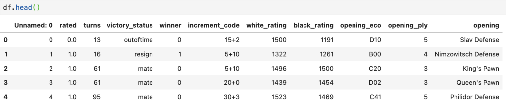
Here’s a preview of the data:
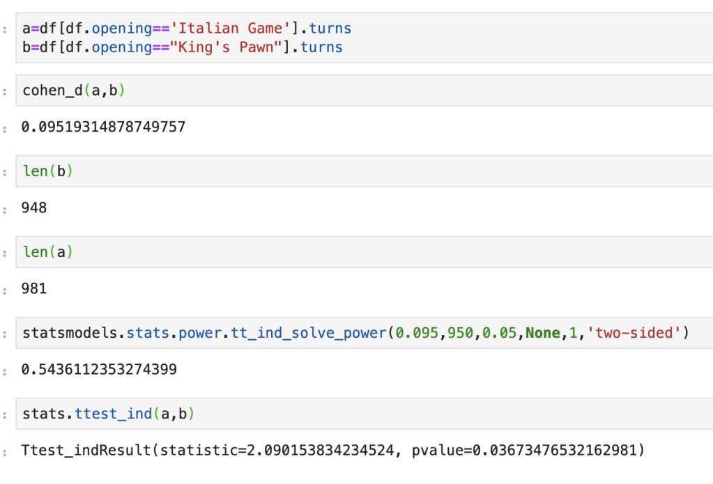
My question is as follows: do games that follow the King’s Pawn process take about as long as games that follow the Italian Game process. Side note: I have no idea what an Italian Game is, or most of the openings listed in the data. We start by looking at effect size. It’s about 0.095, which is pretty low. Next we input the data of turn length from Italian Game processes and King’s Pawn processes. Implicit in this data is everything we need; size, standard deviation, and mean. If we set alpha to 5%, we get a statistical power slightly above 50%. Not great. Running a two-sample-t-test leads to a 3.67% p-value which tells us that these two openings lead to games of differing lengths. The problem is power is low, so it wasn’t quite worth running these tests. And that… is statistical power in action.
Conclusion
Statistical power is important as it can modify how we look at hypothesis tests. If we don’t take a look at power, we may be led to the wrong conclusions. Conversely, when we believe to be witnessing something interesting or unexpected, we can use power to enforce our beliefs.
An examination of the role effect size plays in whether one can trust their tests or not
Introduction
Thanks for visiting my blog today!
Today’s blog concerns statistical power and the role it plays in hypothesis testing. In very simple terms, power is a number between 0% and 100% that tells us how much we are able to trust a statistical test. Let’s say you have never been to southern Illinois, you go there one day in your life, and on that day you witness a tornado. First of all, I’d feel really sorry for you. With this data, though, we might naïvely assume that every day spent in southern Illinois sees a tornado take place. We literally have no other data to refute this claim, so this is, in fact, not that crazy. Except, you know, we only looked at ONE data point. If we had the exact same story, except you saw 500 straight days of tornados, we still have the same ratios of tornados to days spent in southern Illinois, but we now would have confidence in our test if we were to predict that southern Illinois suffers from daily tornados. This is the idea here; just because a statistical test results in a certain outcome, this doesn’t mean that we can immediately trust our result. When people discuss the idea of statistical power, a key metric that helps them make decisions is effect size. Today we’ll discuss effect size and once we understand this concept well, we’ll move on to statistical power.
What is effect size and why does it matter?
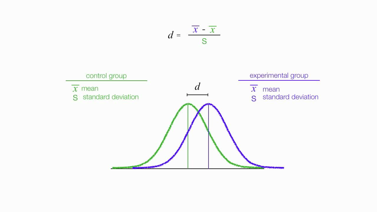
To answer the question above backwards, effect size matters as it is a key input in calculating statistical power. Effect size actually can characterized in a couple different ways in terms of definition. Effect size also has a couple variations on the metrics used. For this post, I will focus on what I believe to be the most common metric and we will also assume that effect size refers to a normalized (transcends units) difference between related groups (usually a control group and a experimental group) in hypothesis testing. In particular, if we are looking at the distribution of two related groups, then we assign the variable known as d (for distance) to the difference between the means in the two distributions. Let’s do a quick example; Let’s say we survey athletes who practice 2 hours a day and people who practice 5 hours a day. The metric d tells us about the difference in how long you practice in terms of effect on production. If we have high effect size, we can assume that more practice has an effect on higher production. Otherwise, it’s may seem like a waste of time to practice 3 extra hours.
How do we calculate effect size?
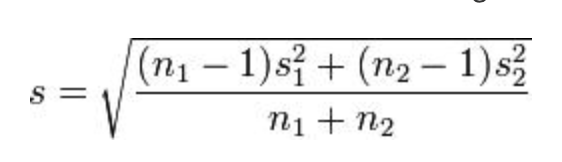
A common way to calculate d is by subtracting the second mean from the first mean and then divide that difference by a pooled standard deviation. The numerator is easy; one mean minus the other. The denominator, though…
It looks messy, but n refers to number of observations while s refers to standard deviation. Each contains a subscript to identify the two distributions. It’s not that bad. It’s a bit of a long and annoying calculation, but by no means complex.
Conclusion
This post introduced gave a gentle and simple understanding of effect size. We discussed the idea and later saw a simple yet descriptive example coupled with an equation to solve for effect size. The follow up to this post will discuss how we take effect size and add it to the statistical power equation to better understand how trustworthy a statistical test may be before we spend time and effort conducting said test.
Understanding the use of z scores in performing statistical inquiries
Introduction
Thanks for visiting my blog today!
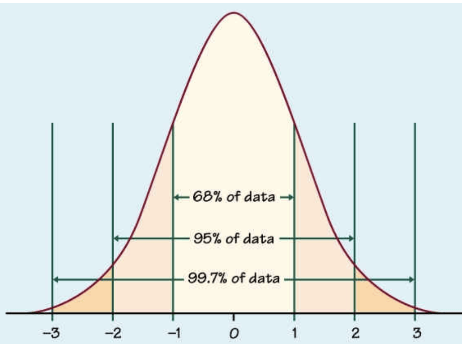
Today’s blog concerns hypothesis testing and the use of z scores to answer questions. We’ll talk about what a z score is, when it needs to be used, and how to interpret the results from a z score-related analysis. While you may or may not be familiar with the term z score, you are very likely to have encountered the normal distribution / bell curve depicted above. I tend to think almost everything in life, like literally everything, is governed by the normal distribution. It’s got a low amount of mass toward the “negative” end, a lot of mass in the middle, and another low amount of mass toward the “positive” side. So if we were to poll a sample of a population on any statistic, say athletic ability, we will find some insane athletes like Michael Phelps or Zach Lavine, some people who are not athletic at all, and everyone else will probably fall into the vast “middle.” Think about anything in life, and you will see the same distribution applies to a whole host of statistics. The fact that this normal / bell-curve is so common and natural to human beings means that people get comfortable using it when trying to answer statistical questions. The main idea of a z score is to see where an observation of data (say IQ of 200, I think that’s a high IQ) falls on the bell curve. If it falls smack in the middle, you are probably not an outlier. On the other hand, if you’re IQ is so high that there is almost no mass at the area of that IQ, we can assume you’re pretty smart. Z scores create a demarkation point that allows us to make use the normal distribution.
When do we even need the z score test in the first place?
We use the z score to see how much a sample from a population represents an outlier. We will need to also use a threshold to decide at what point we call an observation a significant outlier. In hypothesis testing, “alpha” refers to the threshold where we decide whether something is an extreme outlier or not. Often, alpha will be 5%. This means that if the probability of something not being an outlier is 5% or lower, we can assume it is a true outlier. On the standard normal distribution graph (mean zero, standard deviation 1), 5% usually corresponds to 1.96 standard deviations away from the mean of zero. This means if our z score is greater than 1.645 or less than -1.645, we are witnessing a strong outlier. If we have two outliers, we can look at their respective z score to see which outlier is more extreme.
How do we calculate a z score?
It’s actually pretty simple. A z score is equal to the particular observation minus the population mean. That value just described above is then divided by the standard deviation of the population.
Example: if we have a distribution with mean 10 and standard deviation 3, is an observation of 5 a strong outlier? 5-10 = -5. -5/3 = -1.67. So at alpha = 5%, this is a strong outlier. If we restricted alpha and decreased it to 2%, 5 is no longer such a strong outlier. So basically 5 is 1.67 standard deviations from the mean and does represent a significant outlier under alpha at 5%.
If we don’t know the full details of an entire population, things change slightly. Assuming we have more than 30 data points in our sample, the equation becomes observation minus sample (not population) mean. That quantity is then first multiplied by the sample size and then divided by the sample standard deviation.
This process also works if we are trying to evaluate a broader trend. If we want to look at 50 points from a set of 2000 points and see if those 50 points are outliers, we take the mean of 50 points and insert that value as our “observation” input.
Ok, so what happens when we have less than 30 data points? I have another blog to explain what happens there currently in the works.
Conclusion
The z score / z statistic element of hypothesis testing is quite elegant due to its simple nature and connection to the rather natural-feeling normal distribution. It’s an easy and effective tool anyone should have at their disposal whenever trying to perform a meaningful statistical inquiry.
Imposing Structure and Guidelines in Exploratory Data Analysis
Introduction
I like to start off my blogs with the inspiration that led me to write that blog and this blog is no different. I recently spent time working on a project. Part of my general process when performing data science inquiries and building models is to perform exploratory data analysis (EDA from henceforth). While I think modeling is more important than EDA, EDA tends to be the most fun part of a project and is very easy to share with a non-technical audience who don’t know what multiple linear regression or machine learning classification algorithms are. EDA is is often where you explore and manipulate your data to generate descriptive visuals. This helps you get a feel for your data and notice trends and anomalies. Generally, what makes this process exciting is the amount of unique types of visuals and customizations one can use to design said visuals. So now let’s get back to the beginning of the paragraph; I was working on a project and was up to the EDA step. I got really engrossed in this process and spent a lot of effort trying to explore every possible interesting relationship. Unfortunately, however, this soon became stressful as I was just randomly looking around and didn’t really know what I had already covered or at what point I would feel satisfied and therefore planned on stopping. It’s not reasonable to explore every possible relationship in every way. Creating many unique custom data frames, for example, is a headache, even if you get some exciting visuals as a result (and the payoff is not worth the effort you put in). After doing this, I was really uneasy about continuing to perform EDA in my projects. At this point, the most obvious thing in the entire world occurred to me and I felt pretty silly for not having thought of this before; I needed to make an outline and a process for all my future EDA. This may sound counter-intuitive as some people may agree with me that EDA shouldn’t be so rigorous and should be more free-flowing. Despite that opinion from some, that I have the mindset that imposing a structure and plan would be very helpful. Doing this would save me a whole lot of time and stress while also allowing me to keep track of what I had done and capture some of the most important relationships in my data. (I think when some people read this they may not agree with me about my thoughts about an approach to EDA. My response to them is that if there project is mainly focussed on EDA, as opposed to developing a model, then they should understand that this is not the scenario I have in mind. In addition, one still has the ability to impose structure and still perform more comprehensive EDA in the scenario that their project does in fact center around EDA).
Plan
I’m going to provide my process for EDA at a high level. How you decide to interpret my guidelines based on unique scenarios and which visuals you feel best describe and represent your data are up to you. I’d like to also note that I consider hypothesis testing to be part of EDA. I will not discuss hypothesis testing here, but understand that my process can extend to hypothesis testing to a certain degree.
Step 1 – Surveying Data And Binning Variables
I am of the opinion that EDA should be performed before you transform your data using methods such as feature scaling (unless you want to compare features of different average magnitudes). However, just like you would preprocess data for modeling, I believe there is an analogous way to “preprocess” data for EDA. In particular, I would like to focus on binning features. In case you don’t know – feature binning is a method of transforming old variables or generating new variables by splitting up numeric values into intervals. Say we have the data points 1, 4, 7, 8, 3, 5, 2, 2, 5, 9, 7, and 9. We could bin this as [1,5] and (5,9] and assign the labels 0 and 1 to each respective interval. So if we see the number 2 – it becomes a 0. If we see the number 8, however – it becomes a 1. I think it’s a pretty simple idea. It is so effective because often times you will have large gaps in your data or imbalanced features. I talk more about this in another blog about categorical feature encoding, but I would like to provide a quick example. People who buy cars between $300k-$2M probably include the same amount, if not less, than the amount of people buying cars between $10k-$50k. That’s all conjecture and may not in fact be true, but you get the idea. The first interval is significantly bigger than the second in terms of car price range but it is certainly logical to group these two types of people together. You can actually cut your data into bins easily (and assign labels) and even have the choice to cut at quantiles in pandas (pd.cut, pd.qcut). You can also feature engineer before you bin your data using transformations first, and binning second. So this is all great – and will make your models better if you have large gaps… and even give you the option to switch from regression to classification which also can be good – but why do we need to do this for EDA? I think there is a simple answer to this question. You can more efficiently add filters and hues to your data visualizations. Let me give you an example: if you want to find the GDP across all 7 continents (Antarctica must have like a zero GDP) in 2019 and add an extra filter to show large vs. small countries. You would need to add many filters for each unique country size. What a mess! Instead, split companies along a certain population threshold into big and small countries. Now you have 14 data points instead of 200+. 14 = 7 continents * (large population country + small population country). Now I’m sure that some readers can think of other ways to deal with this issue, but I’m just trying to prove a point here, not re-invent the wheel. When I do EDA, I like to first look at violin-plots and histograms to determine how to split my data and how many groups of data (2 bins, 3 bins…) I want, but I also keep my old variables as they are also valuable to EDA as I will allude at later on.
Step 2 – Ask Questions Without Diving Too Deep Into Your Data
This idea will be developed further later on and honestly doesn’t need much explanation right now. Once you know what your data is describing, you should begin to ask legitimate questions you would want to know the answers to and what relationships you would like to explore given the context of your data and write them down. I talk a lot about relationships later on. When you first write down your questions, don’t get too caught up in things like that, just thing about the things in your data you would like to explore using visuals.
Step 3 – Continue Your EDA By Looking At The Target Feature
I would always start an EDA process by looking at the most important and crucial piece of your data – the target feature (assuming it’s labeled data). Go through each of your predictive variables individually and compare them with the target variable with any number of filters you may like. Once you finish up with exploring the relationship with the target variable and variable number one, don’t include variable number one in any more visualizations. I’ll give an example: Say we have the following features: wingspan, height, speed and weight and we wanted to predict the likeliness that any given person played professional basketball. Well, start with variable number one – wingspan. You could see the average wingspan of regular folks versus professional players. However, you could also add other filters such as height to see if the average wingspan of tall professional players vs tall regular people is different. Here, we could have three variables in one simple bar graph: height, wingspan, and the target of whether a player plays professionally or not. You could continue doing this until you have exhausted all the relationships between wingspan, target variable, and anything else (if you so choose). Since you have explored all those relationships (primarily using bar graphs probably) you now can cross off one variable from your list, although it will come back later as we will soon see. Rinse and repeat this process until you go through every variable. The outcome is you have a really good picture of how your target variable moves around with different features as the guiding inputs. This will also give you some insight to reflect on when you run something such as feature importances or coefficients later on. I would like to add one last warning, though. Don’t let this process get out of hand. Just keep a couple visuals for each feature correlation with target variable and don’t be afraid to sacrifice some variables in to keep the more interesting ones. (I realize that there should be a modification to this part of the process if you have above a certain threshold of feature.
Step 4 – Explore Relationships Between Non-Target Features
The next step I usually take is to look at all the data (again), but without including the target feature. Similar to the process described above, if I have 8 non-target features I will think of all the ways that I can compare variable 1 with variables 2 through 8 (with filters). I then look at ways to compare feature 2 with features 3-8 and so on until I am at the comparison between 7 and 8. Now, obviously not every variable may be efficient to compare, easy to compare, or even worth comparing. Here, I tend to have a lot of different types of graphs as I am not focussed on the target feature. You can get more creative than you might be able to when comparing features to the target in a binary target classification problem. There are a lot of articles on how to leverage Seaborn to make exciting visuals and this step of the process is probably a great application of all those articles. I described an example above where we had height, wingspan, weight, and speed (along with a target feature). In terms of the relationships between the predictors, one interesting inquiry, for example, could be the relationship between height and weight in the form of a scatter plot, regression plot, or even joint plot. Developing visuals to demonstrate relationships can also affect your mindset upon filtering out correlation or feature engineering. I’d like to add a Step 4A at this point. When you look at your variables and start writing down all your questions and tracking relationships you want to explore, I highly recommend that you assign certain features as filters only. What I mean by this is the following: Say you have the following (new) example: feature 1 is normally distributed and has 1000 unique values and feature 2 (non-target) has 3 unique values (or distinct intervals). I highly recommend you don’t spend a lot of time exploring all the possible relationships that feature 2 has with other features. Instead, use it as a filter or “hue” (as it’s called in Seaborn). If you want to find the distribution of feature 1, which has many unique values, you could easily run a histogram or violin-plot, but you can tell a whole new story if you filter these data points into three categories dictated by feature 2. So when you write out your EDA plan, figure what works best as a filter and that will save you some more time.
Step 5 – Keep Track Of Your Work
Not much to say about this step. It’s very important though. You could end up wasting a lot of time if you don’t keep track of your work.
Step 6 – Move On With Your Results In Mind
When I am done with EDA, I often switch to hypothesis testing which I like to think as a more equation-y form of EDA. Like EDA, you should have a plan before you start running tests. However, now that you’ve done EDA and gotten a real good feel for your data, you should keep in mind your results for further investigation when you go into hypothesis testing. Say you find a visual that tells a puzzling story – then you should investigate further! Also, as alluded to earlier – your EDA could impact your feature engineering. Really, there’s too much to list in terms of why EDA is such a powerful process even beyond the initial visuals.
Conclusion:
I’ll be very direct about something here: there’s a strong possibility that I was in the minority as someone who often didn’t plan much before going into EDA. Making visuals is exciting and visualizations tend to be easy to share with others when compared to things like a regression summary. Due to this excitement, I used to dive right in without much of a plan beforehand. It’s certainly possible that everyone else already made plans. However, I think that this blog is valuable and important for two reasons. Number 1: Hopefully I helped someone who also felt that EDA was a mess. Number 2: I provided some structure that I think would be beneficial even to those who plan well. EDA is a very exciting part of the data science process and carefully carving out an attack plan will make it even better.
Thanks for reading and I hope you learned something today.
It’s important to keep track of who does and does not show up to work when they are supposed to. I found some interesting data online that gives information on how much work from a range of 0 to 40 hours any employee is expected to miss in a certain week. I ran a couple models and came away with some insights on what my best accuracy would look like and what it would tell me are the most predictive of time expected to miss by an employee.
Process
Collect Data
Clean Data
Model Data
Collect Data
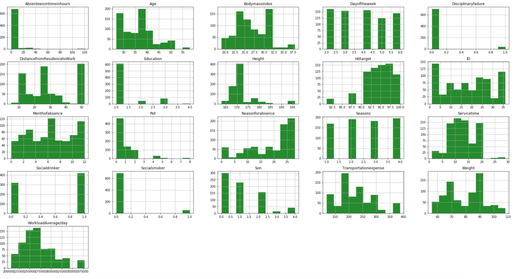
My data comes from the UC Irvine Machine Learning Repository (https://archive.ics.uci.edu/ml/datasets/Absenteeism+at+work). While I will not go through this part in full detail, the link above talks about the numerical representation for “reason for absence.” The features of the data set, other than the target feature of time missed, were: ID, reason for absence, month, age, day of week, season, distance from work, transportation cost, service time, work load, percent of target hit, disciplinary failure, education, social drinker, social smoker, pet, weight, height, BMI, and son. I’m not entirely sure what “son” means. So now I was ready for some data manipulation. However, before I did that, I performed some exploratory data analysis with some custom columns being binning the variables with many unique values such as transportation expense.
EDA
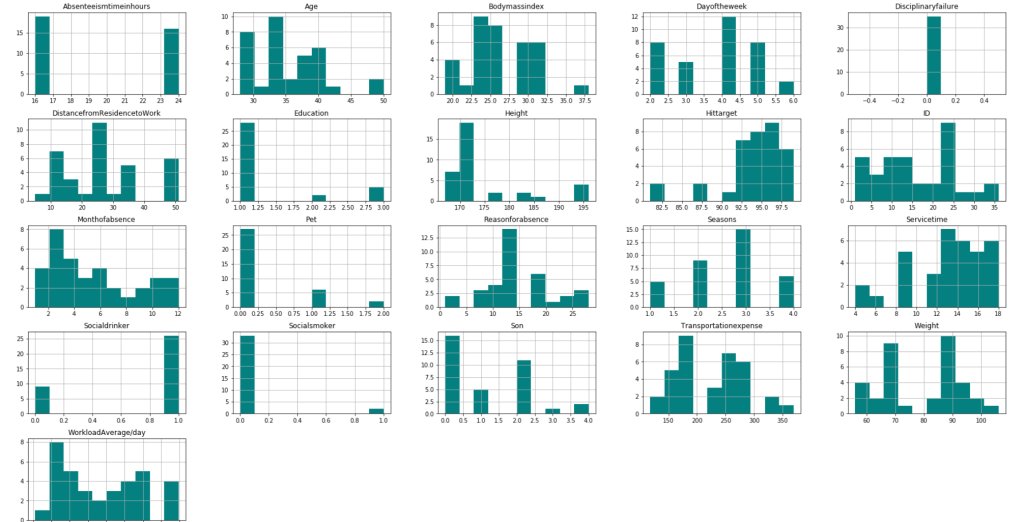
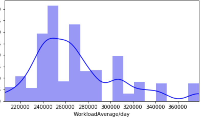
First, I have a histogram of each variable.
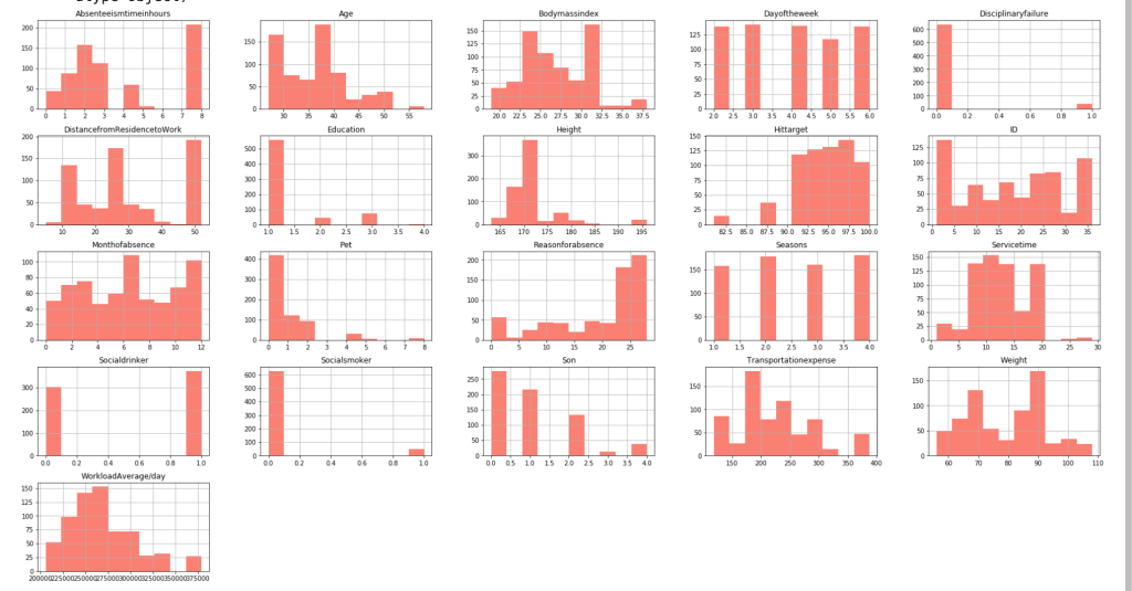
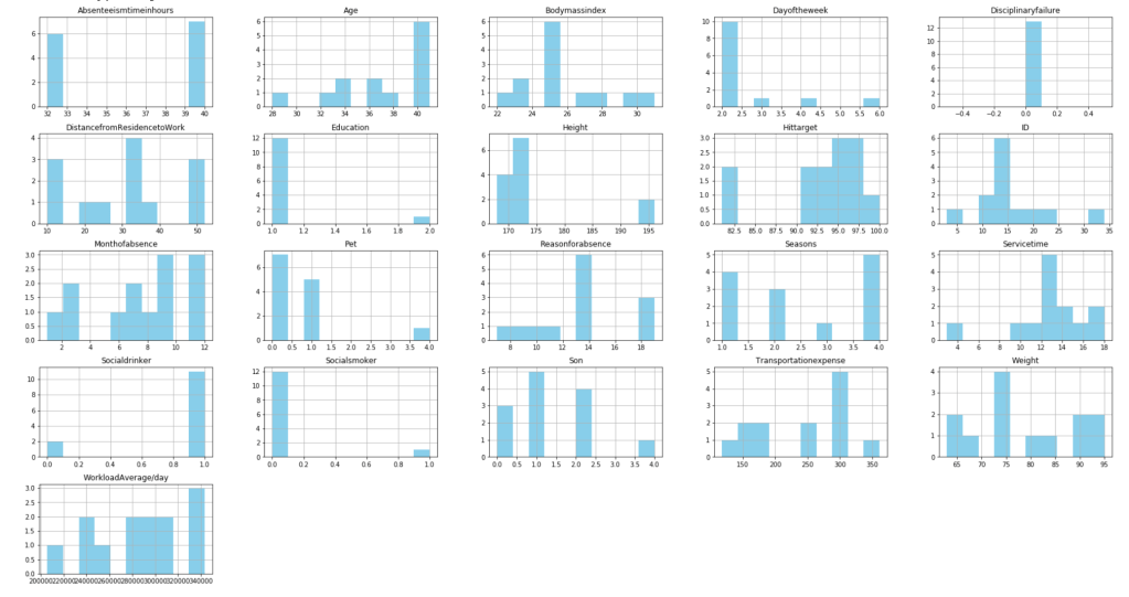
After filtering outliers, the next three histogram charts describe the distribution of variables in cases of missing low, medium, and high amounts of work, respectively.
LowMediumHigh
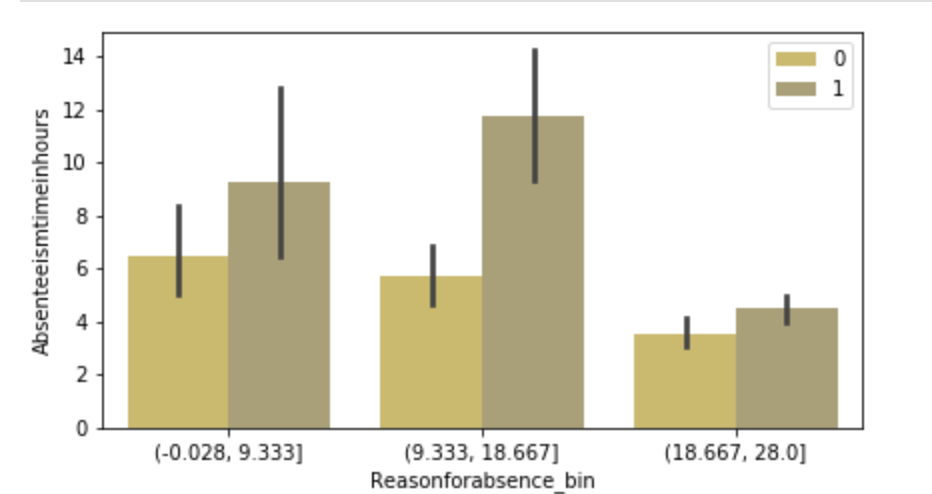
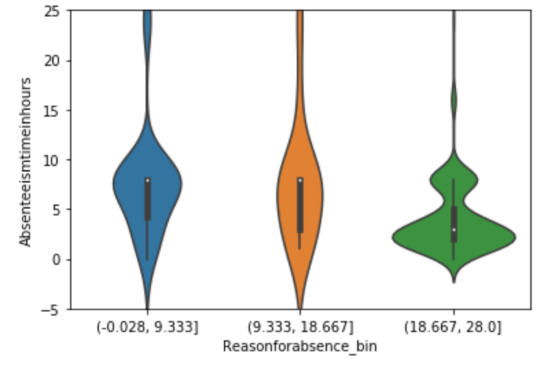
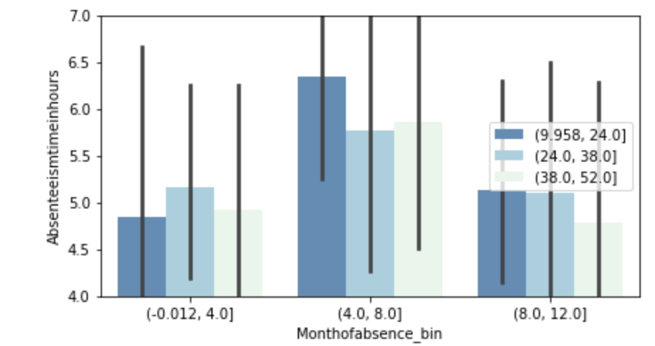
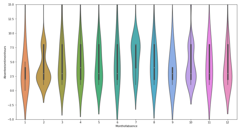
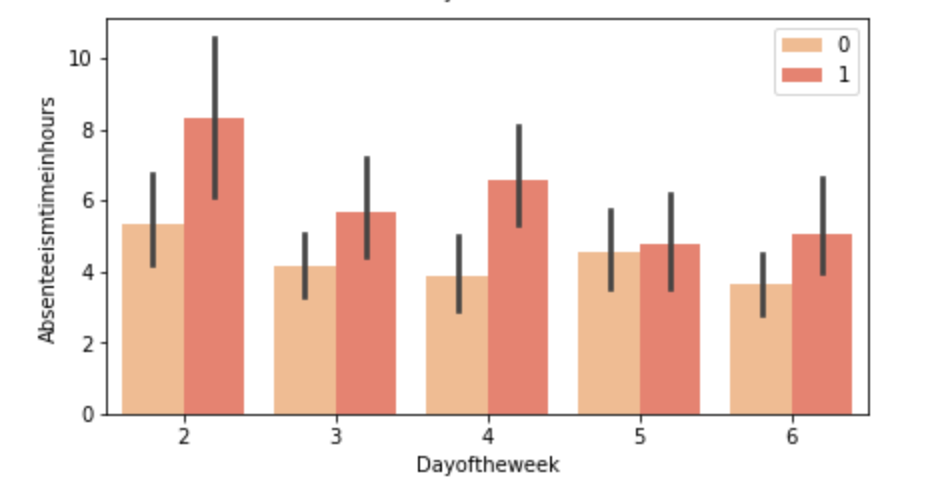
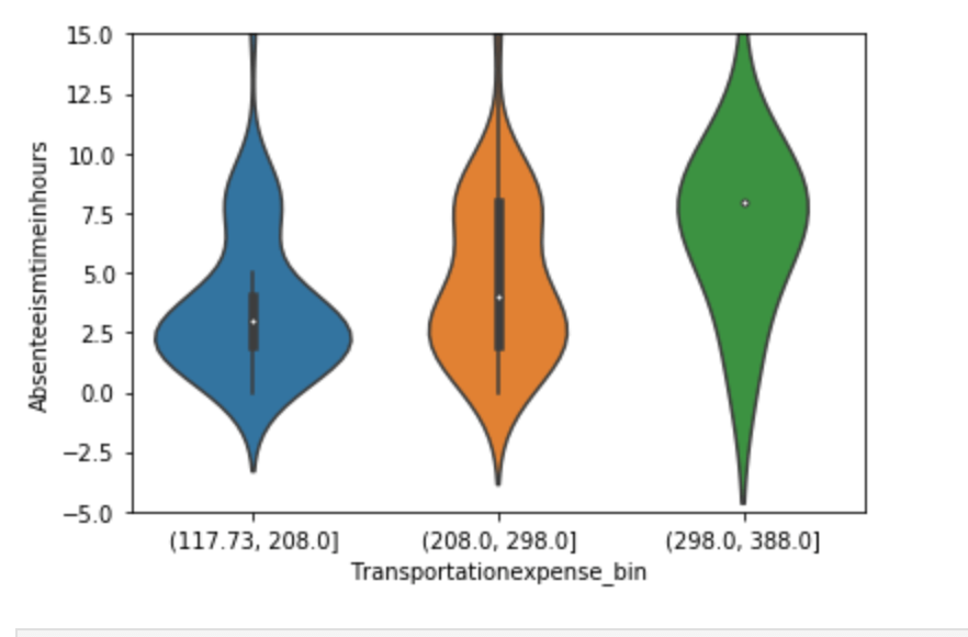
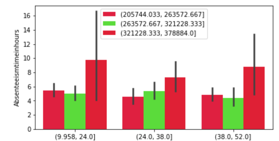
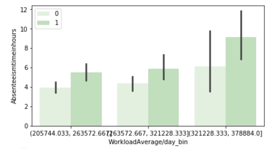
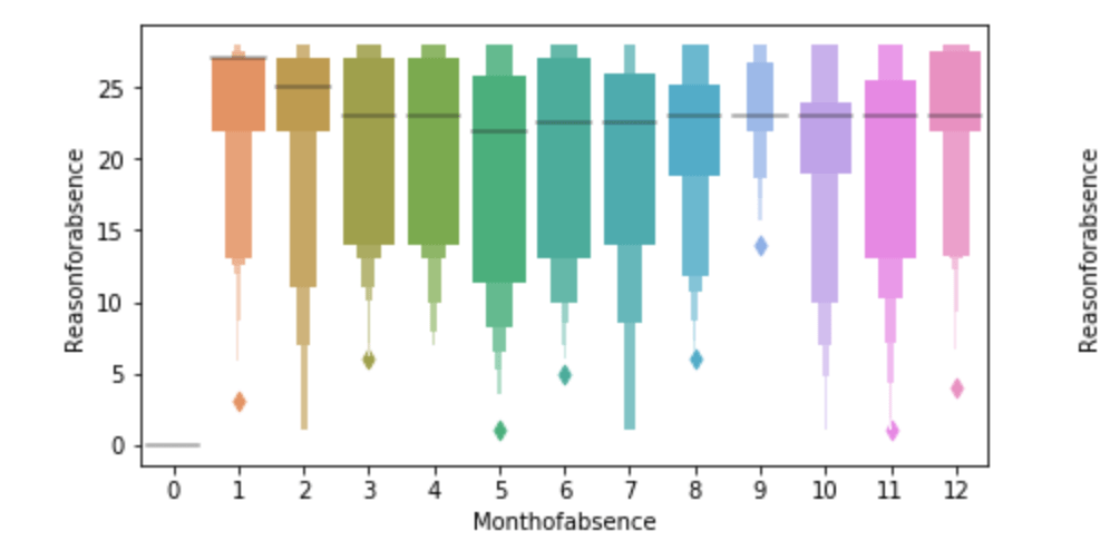
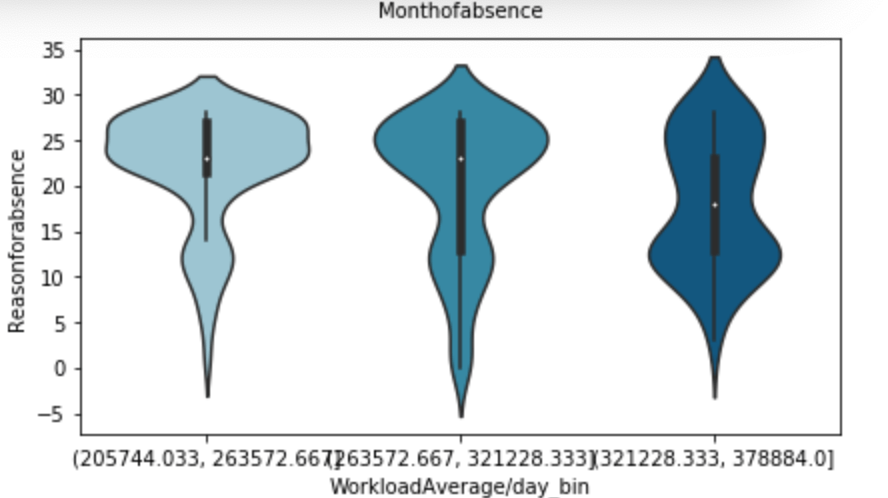
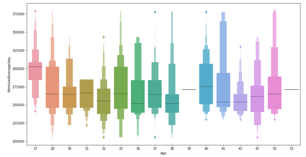
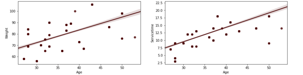
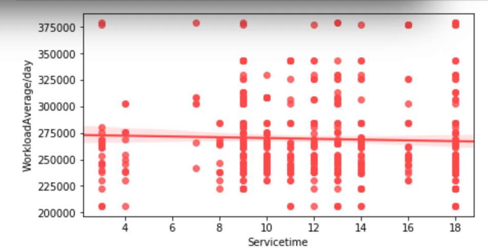
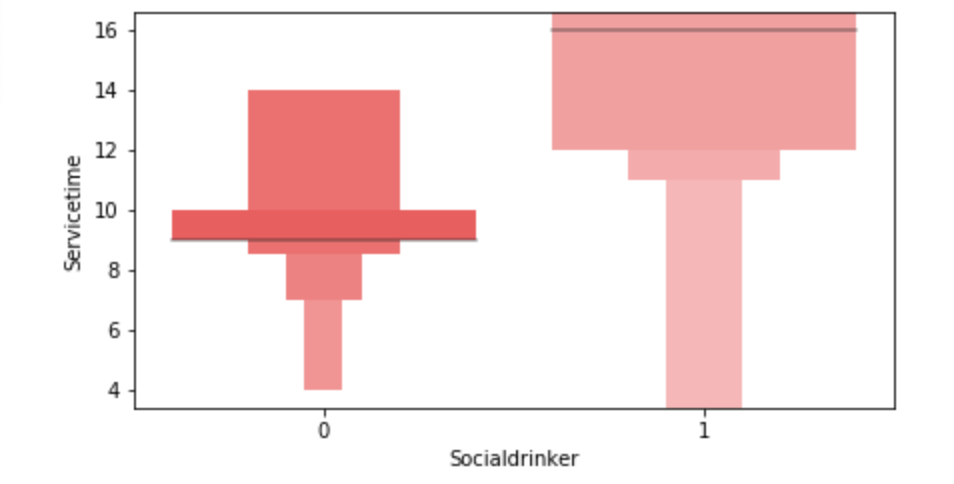
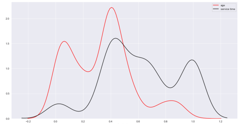
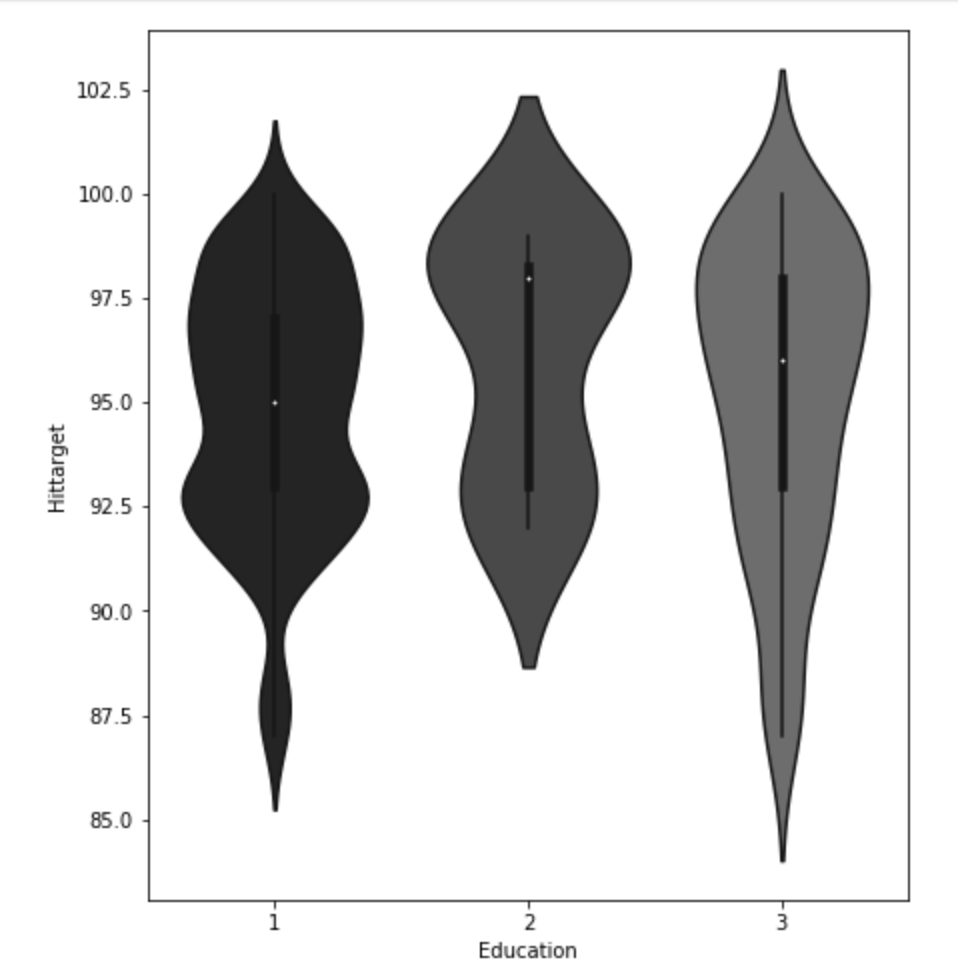
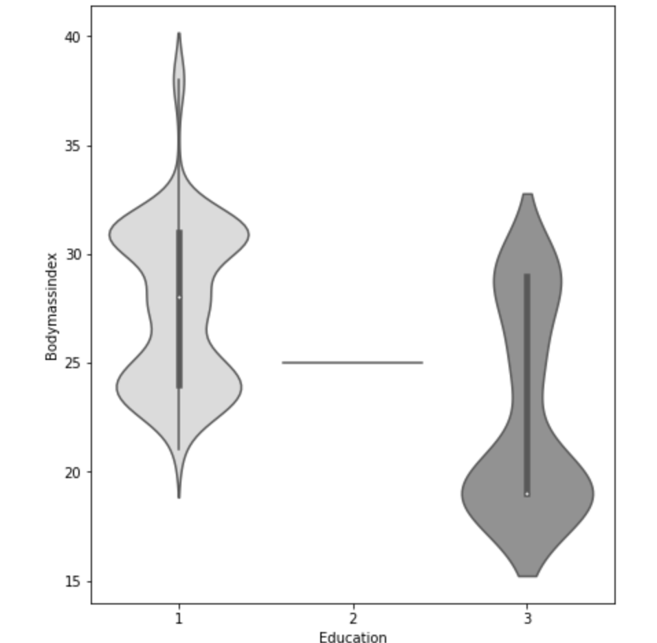
Below, I have displayed a sample of the visuals produced in my exploratory data analysis which I feel tell interesting stories. When an explanation is needed it will be provided.
(O and 1 are binary for “Social Drinker”)(The legend refers distance from work)(O and 1 are binary for “Social Drinker”)(The legend refers transportation expense to get to work)(The legend reflect workload numbers)(O and 1 are binary for “Social Drinker”)Histogram(Values adjusted using Min-Max scaler)
This concludes the EDA section.
Hypothesis Testing
I’ll do a quick run-through here of some of the hypothesis testing I performed and what I learned. I examined the seasons of the year to see if there was a discrepancy in the absences observed in the Summer and Spring vs Winter and Fall. What I found was that there wasn’t much evidence to say a difference exists. I found with high statistical power that people with higher travel expenses tend to miss more work. This was also the case with people who have longer distances to work. Transportation costs as well as distance to work also have a moderate effect on service time at a company. Age has a moderate effect on whether people tend to smoke or drink socially but not enough to have statistical significance. In addition, there appears to be little correlation with time at the company and whether or not targets were hit. However, this test has low statistical power and has a p-value that is somewhat close to 5% implying that an adjusted alpha may change how we view this test both in terms of type 1 error and statistical power. People with less education tend to drink more as well. Education has a moderate correlation with service time. Anyway, that is very quick recap of the main hypotheses I tested boiled down to the most easy way to communicate their findings.
Clean Data
I started out by binning variables with wildly uneven distributions. Next, I used categorical data encoding to encode all my newly binned features. Next, I applied scaling so that all the data would be within 3 standard deviations of each variable’s mean. Having filtered out misleading values, I binned my target variable into three groups. Next, I removed correlation. I will go back and discuss some of these topics later in this blog when I discuss some of the difficulties I faced.
Model Data
My next step was to split and model my data. One problem came up. I had a huge imbalance among my classes. The “lowest amount of work missed” class had way more than the other two classes. Therefore, I synthetically created new data to have every class have the same amount of cases. To find my most ideal model and then improve it… well I first needed to find the best model. I applied 6 types of scaling across 9 models = 54 results and found that my best model would be a Random Forest model. I even found that adding polynomial features would give me near 100% accuracy on training data without much loss on test data. Anyway, I went back to my random forest model. I found the most indicative features of time missed in order from biggest indicator to smallest indicator were: month, reason for absence, work load, day of the week, season, and social drinker. There are obviously other features, but these are the most predictive ones. The others provide less information.
Problems Faced in Project
The first problem I had was not looking at the distribution of the target variable. It is a continuous variable, however, there are very few values in certain ranges. I therefore split it into three bins; missing little work, a medium amount of work, and a lot of work. I also experimented with having two bins as well as different cutoff points to pick the bins, but three bins worked better. This also affected my upsampling as the different binning methods resulted in different class breakdowns. The next problem I had was a similar one. How would I bin variables? In short, I tried a couple of ways and found that three bins worked well. All this binning was not done using quantiles, by the way. That would imply no target class imbalance which was not the case. I tried using quantiles, but did not find it effective. I also experimented with different categorical feature encoding but found that the most effective method was to bin based on mean value in connection with target variable (check my home page for a blog about that concept). I ran a gridsearch to optimize my random forest at the very end and then printed a confusion matrix. This was not good, but I nee to be intellectually honest. Predicting when someone would fall into class 0 (“missing low amount of work”) my model was amazing and its recall exceeded precision. However, it did not work well on the other two. Now keep in mind that you do not upsample test data and this could be a total fluke. However, that was still frustrating to see. An obvious next step is to collect more data and continue to improve the model. One last idea I want to talk about is exploratory data analysis. Now, to be fair, this could be inserted into any blog. Exploratory data analysis is both fun and interesting as it allows you to be creative and take a dive into your idea using visuals as quick story-tellers. The project I had just scrapped before acquiring the data for this project drove me kind of crazy because I didn’t really have a plan for my exploratory data analysis. It was arbitrary and unending. That is never a good plan. EDA should be planned and thought out. I will talk more / have talked more about this (depending on when you read this blog) in another blog but the main point is you want to think of yourself as person who doesn’t do programming who just wants to ask questions based on the names of the features. Having structure in place for EDA is less free-flowing and exciting than not having structure, but it ensures that you work efficiently and have a good start point as well as stop point. That really helped me save a lot of stress.
Conclusion
It’s time to wrap things up. At this point, I think I would need more data to continue to improve this project, and I’m not sure where that data would come from. In addition, there are a lot of ambiguities in this data set such as the numerical choices for reason for absence. Nevertheless, I think that by doing this project I learned how to create an EDA process and how to take a step back and rephrase your questions as well as rethink your thought process. Just because a variable is continuous, this does not imply it requires regression analysis. Think about your statistical inquiries as questions, think about what makes sense from an outsider’s perspective, and then go crazy!