An examination of the role effect size plays in whether one can trust their tests or not

Introduction

Thanks for visiting my blog today!

Today’s blog concerns statistical power and the role it plays in hypothesis testing. In very simple terms, power is a number between 0% and 100% that tells us how much we are able to trust a statistical test. Let’s say you have never been to southern Illinois, you go there one day in your life, and on that day you witness a tornado. First of all, I’d feel really sorry for you. With this data, though, we might naïvely assume that every day spent in southern Illinois sees a tornado take place. We literally have no other data to refute this claim, so this is, in fact, not that crazy. Except, you know, we only looked at ONE data point. If we had the exact same story, except you saw 500 straight days of tornados, we still have the same ratios of tornados to days spent in southern Illinois, but we now would have confidence in our test if we were to predict that southern Illinois suffers from daily tornados. This is the idea here; just because a statistical test results in a certain outcome, this doesn’t mean that we can immediately trust our result. When people discuss the idea of statistical power, a key metric that helps them make decisions is effect size. Today we’ll discuss effect size and once we understand this concept well, we’ll move on to statistical power.

What is effect size and why does it matter?

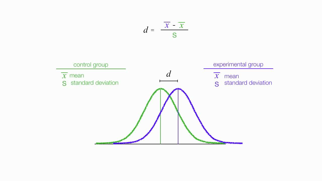
To answer the question above backwards, effect size matters as it is a key input in calculating statistical power. Effect size actually can characterized in a couple different ways in terms of definition. Effect size also has a couple variations on the metrics used. For this post, I will focus on what I believe to be the most common metric and we will also assume that effect size refers to a normalized (transcends units) difference between related groups (usually a control group and a experimental group) in hypothesis testing. In particular, if we are looking at the distribution of two related groups, then we assign the variable known as d (for distance) to the difference between the means in the two distributions. Let’s do a quick example; Let’s say we survey athletes who practice 2 hours a day and people who practice 5 hours a day. The metric d tells us about the difference in how long you practice in terms of effect on production. If we have high effect size, we can assume that more practice has an effect on higher production. Otherwise, it’s may seem like a waste of time to practice 3 extra hours.

How do we calculate effect size?

A common way to calculate d is by subtracting the second mean from the first mean and then divide that difference by a pooled standard deviation. The numerator is easy; one mean minus the other. The denominator, though…

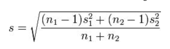
It looks messy, but n refers to number of observations while s refers to standard deviation. Each contains a subscript to identify the two distributions. It’s not that bad. It’s a bit of a long and annoying calculation, but by no means complex.

Conclusion

This post introduced gave a gentle and simple understanding of effect size. We discussed the idea and later saw a simple yet descriptive example coupled with an equation to solve for effect size. The follow up to this post will discuss how we take effect size and add it to the statistical power equation to better understand how trustworthy a statistical test may be before we spend time and effort conducting said test.