Using a sample data set to create and test a decision tree model.

Introduction

Welcome to my blog and thanks for dropping by!

Today, I have my second installment in my decision tree blog series. I’m going to create and run a model leveraging decision trees using data I found on a public data repository. Hopefully you saw part one in this series as it will be pretty important. For a quick reminder, I am going to use the gini metric to make my tree. Let’s begin!

Data Preparation

My data concerns wine quality. I picked this data set because it was a relatively basic data set and was pretty clean to begin. My only important preprocessing was running feature selection to cut down from ten features to five predictive feature. I also binned all my features as either a zero or one to make life easier. That means that instead of having a continuous measure between, say 1 and 100, it instead becomes 0 for lower and 1 for higher. Thankfully, this did not sacrifice model accuracy that much. Also, just to keep things simple, I decided to only look at 150 rows of data so things don’t get out of control. I also wrote the following function for calculating gini:

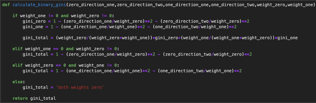
Here is a function that is built on top of that function just to make things a bit easier (it was cut off a bit):

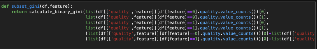
The function above will allow me to easily go into different branches of each tree while doing very little manual computer programming.

Anyway, this is going to get a little messy I imagine. I will use my functions to skip the annoying calculations and data manipulation, but there are still going to be a lot of branches. Therefore, I will try to provide a picture of my hand-typed tree. (I found this link for how to create a visualization using python: https://towardsdatascience.com/visualizing-decision-trees-with-python-scikit-learn-graphviz-matplotlib-1c50b4aa68dc).

By the way… here is a preview of my data containing five predictive features:

Building My Tree

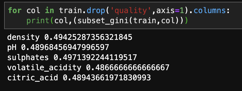
Let’s start with the base gini values for the five predictive features in terms of their effect on the target feature of quality.

Now, we enter the volatile acidity 0 and volatile acidity 1 worlds:

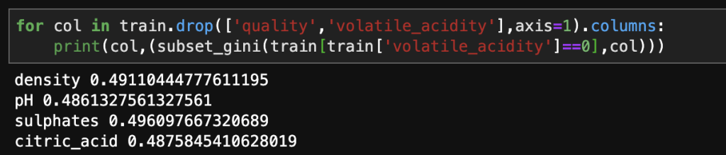
Ok, so what does all this mean? Assuming we take the value of zero for volatile acidity, and as we’ll see – that is the far more interesting path, our next branch to look at would be pH. Afterward we dive into pH 1 and pH 0 and so on…

Now that we have got a feel of what this tree is going to look like in terms of how we set up our calculations along each branch, I am going to just do the rest by myself and post some final results. There are going to be a lot of branches and looking at every single one will get boring very quickly.

A couple notes:

One: part of this project involved upsampling a minority target class. I did a whole lot of work and basically finished my tree but had to do it all over again because of target class imbalance. Don’t neglect about this key part of the modeling process (if necessary) or your models will be incomplete and inacurate!

Two: I am going to post my model in the form of an Excel table showing all the paths of the tree. You will most likely have no way of knowing this, unless you look at the data (https://www.kaggle.com/uciml/red-wine-quality-cortez-et-al-2009) and go through the same pre-processing I did (which was rather non-traditional), but not all the subsets displayed actually exist. So I will have some branches from the tree written out in my Excel table that are not actually part of any tree at all. When that happens, I took a step back and just saw what things would look like in the absence of that feature. Some combinations of characteristics of wine (that’s what my data concerns) don’t exist in the 150 rows I chose at random to build my tree. Consequently, when you view my tree, you should focus on the order of features as opposed to the particular combinations, as I imagine that I will end up listing every possible combination possible. The order that the features appear tell the story of what feature was most predictive at each branch. Don’t get lost in all the details.

Here is what I came up with (I color coded each feature to make it easy to follow):

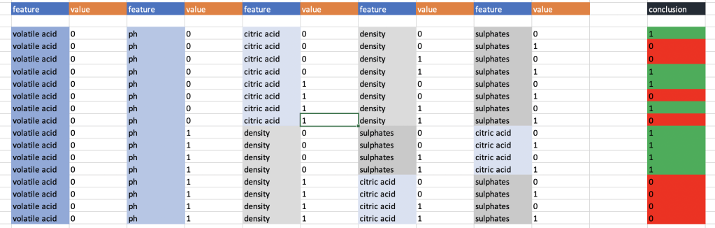
In case you are wondering, the first feature in my tree, volatile acidity, was so predictive that any time it was equal to 1, the conclusion was 0 for the target variable.

So now it’s time to see if this actually works; we need test data. I used a basic train-test-split. That’s data science for language for artificially separating data to specifically not build a model on and instead use for testing purposes. I’ll be transparent and display my test data set. At this point, I don’t know how well my model is going to work so we’re all in this together in a sense.

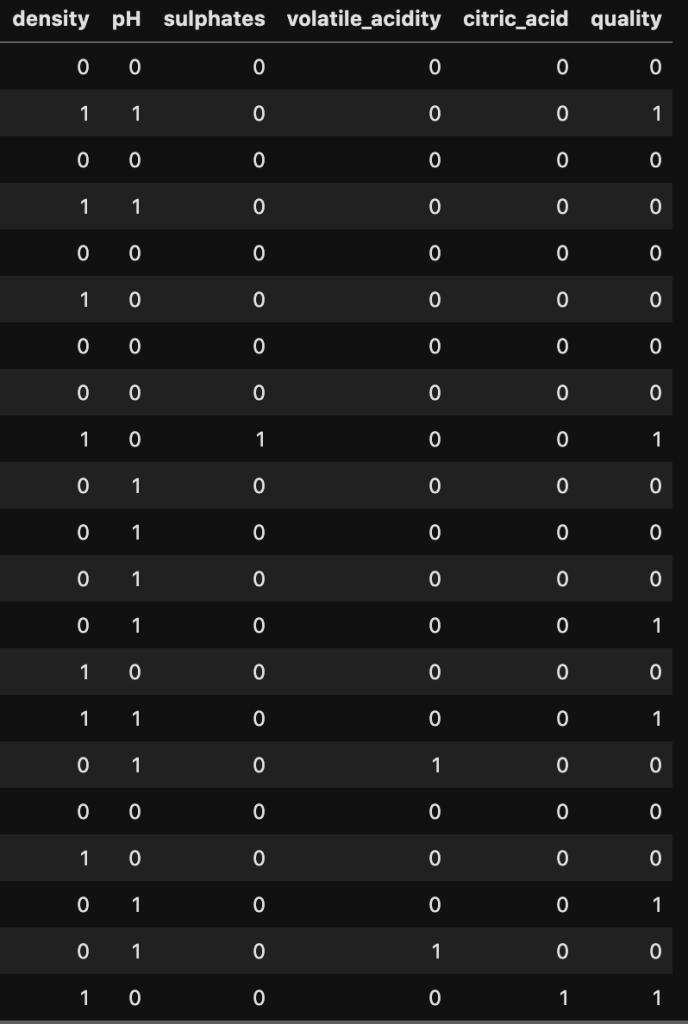
So now that we have the logic in place and you have seen all my test data, you could theoretically “run the model” yourself and follow each path outlined above and see how the data fits in. That sounds like a lot of work, though. Here is what it would look like if you did all that work:

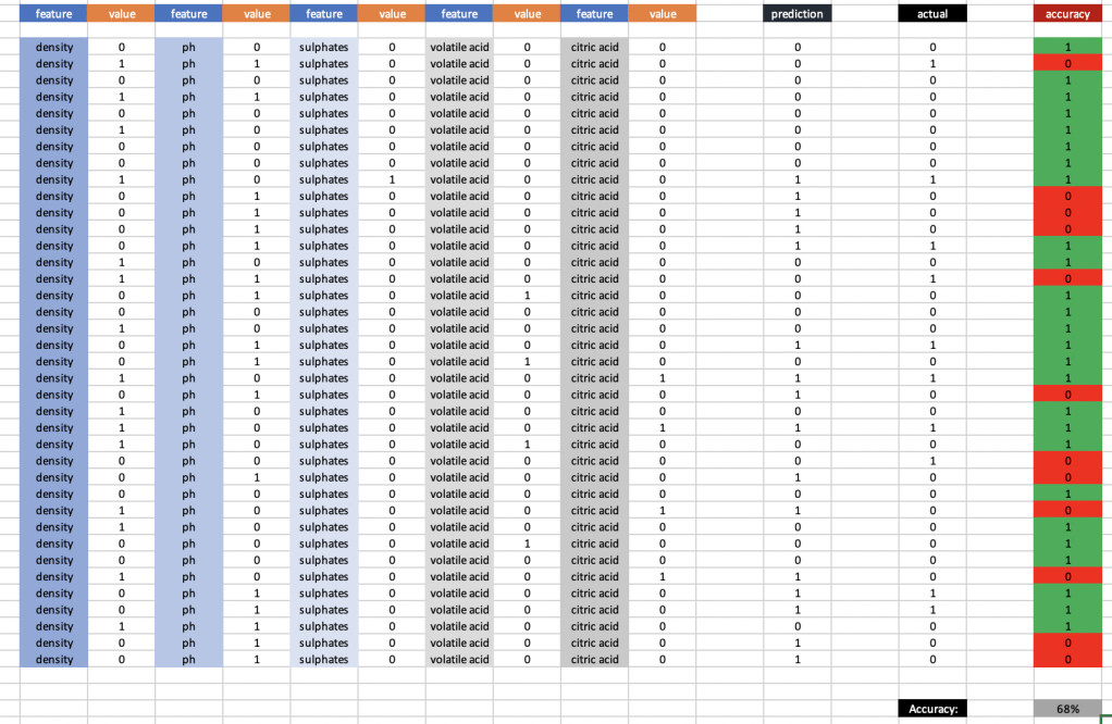
At 68% accuracy, I am proud of this model. If we eliminate the binary binning and add more of the original data, this number will go up to ~77%.

Conclusion

Using the gini metric and a real data set (and a little bit of preprocessing magic), we were able to create a basic decision tree. Considering the circumstances, it was fairly accurate. Decision trees are great because they are fairly simple conceptually and the math is not that hard either.

Thanks for reading!