Understanding how to build a decision tree using statistical methods.

Introduction

Thanks for visiting my blog today!

Life is complex and largely guided by the decisions we make. Decisions are also complex and are usually the result of a cascade of other decisions and logic flowing through our heads. Just like we all make various decision trees in our heads (whether we actively think about them or not) to guide our decisions, machines can also leverage a sequence of decisions (based on logical rules) to come to a conclusion. Example: I go to a Blackhawks game. The Blackhawks are tied with 2 minutes left. It’s a preseason game. Do I leave early to avoid the parking lot they call “traffic” and catch the rest on TV or radio, or do I stay and watch a potential overtime game (which is always exciting). There’s nothing on the line for the Blackhawks (and therefore their fan base) but I paid money and took a chunk of time out of my day to see Patrick Kane light up the scoreboard and sing along to Chelsea Dagger. There are few experiences that are as exciting as a last second or overtime / extra-time game winning play and I know from past live experience. Nevertheless, we are only scratching the surface of what factors may or may not be at play. What if I am a season ticket holder? I probably would just leave early. What if I come to visit my cousins in Chicago for 6 individual (and separate) weeks every year? I might want to stay as it’s likely that some weeks I visit there won’t even be a game. Right there, I built a machine learning model in front of your eyes (sort of). My de-facto features are timeInChicago, futureGamesAttending, preseasonSeasonPosteason, timeAvailable, gameSituation. (These are the ones I made up after looking back at build-up to this point and think they work well – I’m sure others will think of different ways to contextualize this problem). My target feature can be binary; stay or leave. It can also be continuous; time spent at game. It can also be multi-class; periods stayed in (1, 2, or 3). This target feature ambiguity can change the problem depending on one’s philosophy. Whether you realize this or not, you are effectively creating a decision tree. It may not feel like all these calculations and equations are running through your head and you may not even take that long or incur that much stress when making a decision, but you’re using that decision tree logic.

In today’s blog we are going to look at the concepts surrounding a decision tree and discuss how they are built and make decisions. In my next blog in this series (which may or may not be my next blog I write), I will take the ideas discussed here and show an application on real-world data. Following that, I will build a decision tree model from scratch in python. The blog after that will focus on how to take the basic decision tree model to the next level using a random forest. After that blog, I will show you how to leverage and optimize decision trees and random forests in machine learning models using python. There may be more on the way, but that’s the plan for now.

I’d like to add that I think I’m going to learn a lot myself in this blog as it’s important, especially during a job interview, to explain concepts. Many of you who may know python may know ways to quickly create and run a decision tree model. However, in my opinion, it is equally as important (if not more) to understand the concepts and to be able explain what things like entropy and information gain are (some main concepts to be introduced later). Concepts generally stay in place, but coding tends to evolve.

Let’s get to the root of the issue.

How Do We Begin?

It makes sense that we want to start with the most decisive feature. Say a restaurant only serves ribeye steak on Monday. I go to the restaurant and have to decide what to order, and I really like ribeye steak. How do I begin my decision tree? The first thing I ask myself is if it’s Monday or not. If it’s Monday, I will always get the steak. Otherwise, I won’t be able to order that steak. In the non-Monday universe, aka the one where I will be guaranteed to not get the steak, the whole tree changes when I pick what to eat. So we want to start with the most decisive features and work our way down to the least decisive features. Sometimes the trees will not have the same branches at the same time. Say the features (in this restaurant example) are day of the week, time of day, people with me eating, and cash in my pocket. Now I really like steak. So much so that every Monday I am willing to spend any amount of money for the ribeye steak (I suppose in this example, the cost is variable). For other menu items, I may concern myself with price a bit more. Price doesn’t matter in the presence of value but becomes a big issue in the absence of value. So, in my example: money in pocket will be more decisive in the non-Monday example than the Monday example and therefore find itself at a different place in the tree. The way this presents itself in the tree is that 100% of the times it is Monday and I have the cash to pay for the steak I will pay for it and 100% of the time I don’t quite have enough in my pocket I will have to find some other option. That’s how we start each branch of the tree, starting with the first branch.

How Do We Use Math To Solve This Problem?

There’s a couple ways to go about this. For today, I’d like to discuss gini (pronounced the same as Ginny Weasley from Harry Potter). Gini is a measure of something called impurity. Most of the time, with the exception of my Monday / steak example, we don’t have completely decisive features. Usually there is variance within each feature. Impurity is the amount of confusion or lack of clarity in the decisiveness of a feature. So if we have a feature that has around 50% of the occurrences resulting in outcome 1 and 50% resulting in outcome 2, we have not learned anything exciting. By leveraging the gini statistic, we can understand which of our features is least impure and start the tree with that feature and then continue the tree by having the next branch be whatever is least impure in reference to the previous branch. So here is the equation we have all been waiting for:

Here’s a quick example, and then I’ll get back to the equation (I apologize for the rotation):

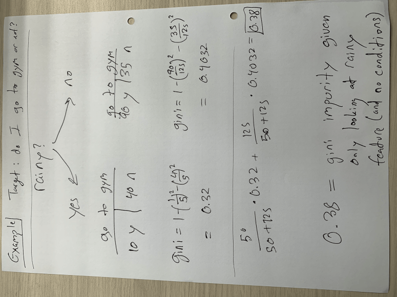
In the example above, I only compare the target feature to whether it’s rainy or not. There is no conditional probability here on things like time of day or day of week. This implies that we are at (or deciding) the top of the tree and seeing if raininess is as strong a predictive feature as other ones. We see that if we assume it is rainy, our gini impurity, as measured by one minus the probability of yes and the probability of no (both squared), sits around 0.32. If it is not a rainy day, the gini impurity is a bit higher, meaning we don’t have as much clarity as to whether or not I will go to the gym. In the weighted average result of 0.38, we see that this number is close to 0.4 than 0.32 because most days are not rainy days. In my opinion, using this data generated on the spot for demonstration purposes, the gini impurity for raniness is quite high and therefore would not sit at the top of the tree. It would be a lower branch. This concept is not exclusive to the binary choice, however it presents itself differently in other case. Say we want to know if I go to the gym based on how much free time I have in my day and my options include a range of numbers such as 60 minutes, 75 minutes, 85 minutes, and other values. To decide how we split the tree, we create “cutoff” points (corresponding to each value – so we create a cutoff at over 67.5 minutes and below 67.5 minutes followed by testing the next cutoff at over 80 minutes and below 80 minutes) to find the “cutoff” point with the least impurity. In other words, if we assume that the best way to measure whether I go or not is by deciding if I have more than 80 minutes free or less than 80 minutes free, than the tree goes on to ask if I have more than 80 minutes or less than 80 minutes. I also think this means that the cutoff point can change in different parts of the tree. For example, the 80 minute concept may be important on rainy days but I may go to the gym even with less free time on sunny days. Note that the cutoff always represents a binary direction forward. Basically we keep following the decision tree down using gini as a guide until we get to the last feature. At that point we just use the majority to decide.

Conclusion

Decision trees are actually not that complex, they can just take a long time when you have a lot of data. This is great to know and quite comforting considering how fundamental they implicitly are to everyday life. If you’re ever trying to understand the algorithm, explain it in an interview, or make your own decision tree (for whatever reason…), I hope this has been a good guide.

Thanks for reading!