Simple Multiple Linear Regression in Python

Introduction

Thank you for visiting my blog!

Today, I’m going to be doing the third part of my series in linear regression. I originally intended to end on part 3, but I have considered continuing with further blogs. We’ll see what happens. In my first blog, I introduced the concepts and foundations of linear regression. In my second blog, I talked about one topic often correlated to linear regression known as gradient descent. In many ways, this third blog represents the most exciting blog in the series, but also the shortest and easiest to compose blog. Why? The answer is that I hope to empower and inspire anyone with even moderate interest in python to perform meaningful analysis using linear regression. We’ll soon see that once you have the right framework, it is a pretty simple process. Now, keep in mind that the regression I will display is about as easy and simple as it gets. The data I chose was clean and based on what I had seen online, was not that complex. So pay attention to the parts that allow you to perform regression and not the parts that relate to data cleaning.

Data Collection

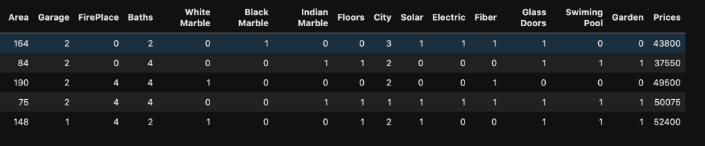
My data comes from kaggle.com and can be found at (https://www.kaggle.com/greenwing1985/housepricing). The data (which I think is not from a real world data set) talks about house pricing with features including (by name): area, garage, fire place, baths, white marble, black marble, Indian marble, floors, city, solar, electric, fiber, glass doors, swimming pool, and garden. The target feature was price.

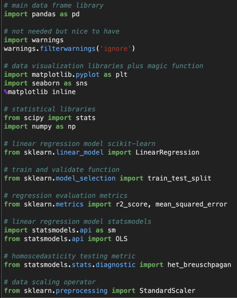
Before I give you screenshots with data, I’d like to provide all the necessary imports for python (plus some extra ones I didn’t use but are usually quite important).

Here’s a look at the actual data:

Here is a list of how many null values occur in each variable as well as each variable’s data type

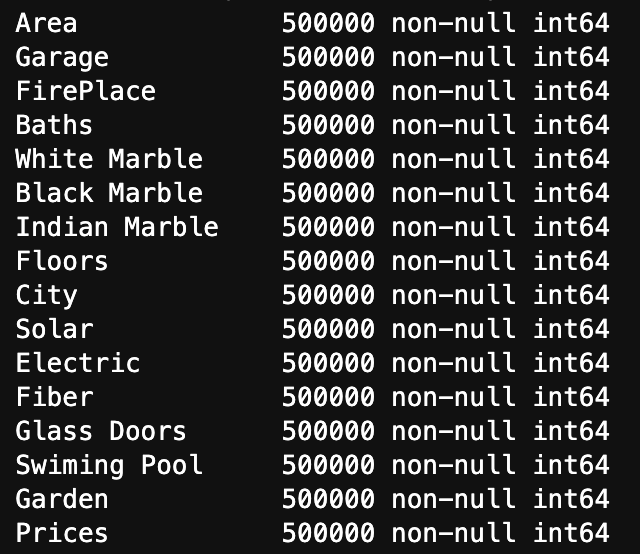
We see three key observations here. One is that we have 500000 rows of each value. Two is that we have no null values. Finally, three is that they are all represented using integers.

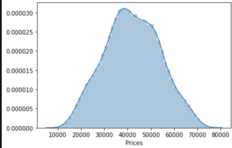
One last observation: the target class seems to be normally distributed to some degree.

Linear Regression Assumptions

Linearity

Conveniently, most of our data consists of discrete features with values consisting of whole numbers between 1 and 5. That makes life somewhat easier. The only feature to really test was area. Here goes:

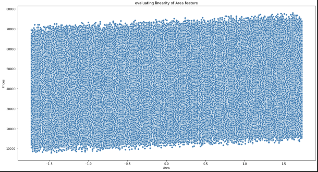
This is not the most beautiful graph. I have however, concluded that it satisfies linearity and have confirmed this conclusion with others who look at this data.

Multicollinearity

Do features correlate highly to each other?

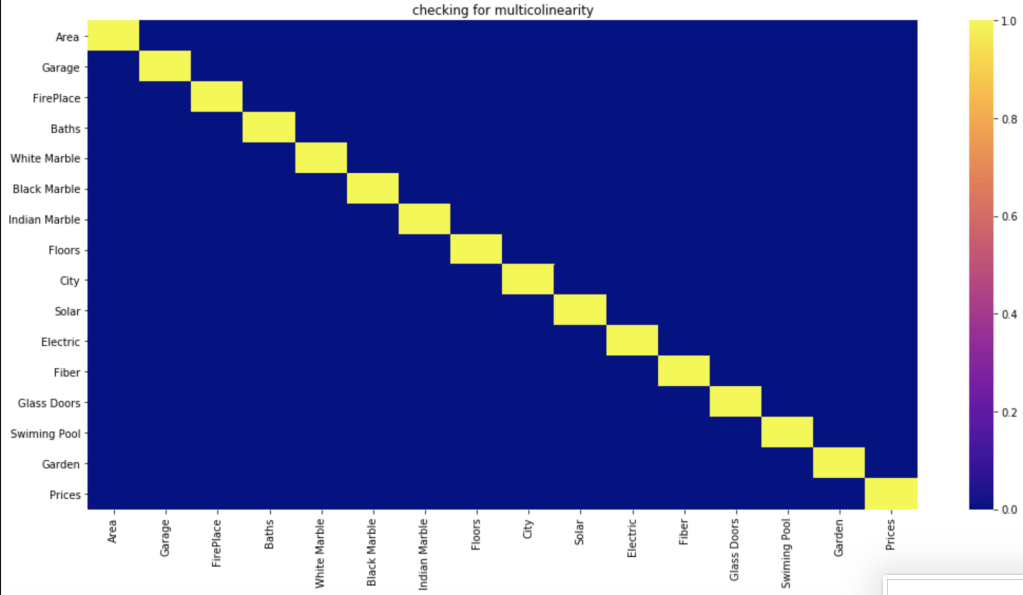
Based on a filter of 70%, which is common, it seems like the features have no meaningful correlation with each other.

Normal Distribution of Residuals

First, of all the average of residuals is around zero, so that’s a good start. I realize that the following graph is not the most convincing visual but I was able to confirm that this assumption is satisfied.

Homoscedasticity

I’ll be very honest, this was a bit of a mess. In the imports above I show an import for the Breusch-Pagan test (https://en.wikipedia.org/wiki/Breusch%E2%80%93Pagan_test). I’ll save you the visuals, as I didn’t find them convincing. However, my conclusions appeared to be right as they were confirmed in the kaggle community. So, in the end there was homoscedasticity present.

Conclusion

We have everything we need to conduct linear regression.

Data Preparation

To prepare my data, all I used was standard scaling. I have a blog on that if you’d like more information (https://data8.science.blog/2020/05/06/feature-scaling/).

Statsmodels Method

There are two primary methods of linear regression. One is by using statsmodels and the other one is by using sklearn. I don’t know how to split data in statsmodels and later evaluate on other data, in a quick way, at least within statsmodels. That said, statsmodels gives a more comprehensive summary as we are about to see. So there is a tradeoff between which package you choose. You’ll soon see what I mean in more detail. In three lines of code, I am going to create a regression model, fit the regression, and check results. Let’s see:

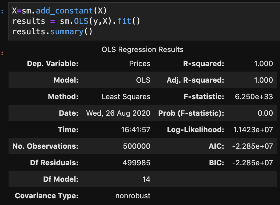
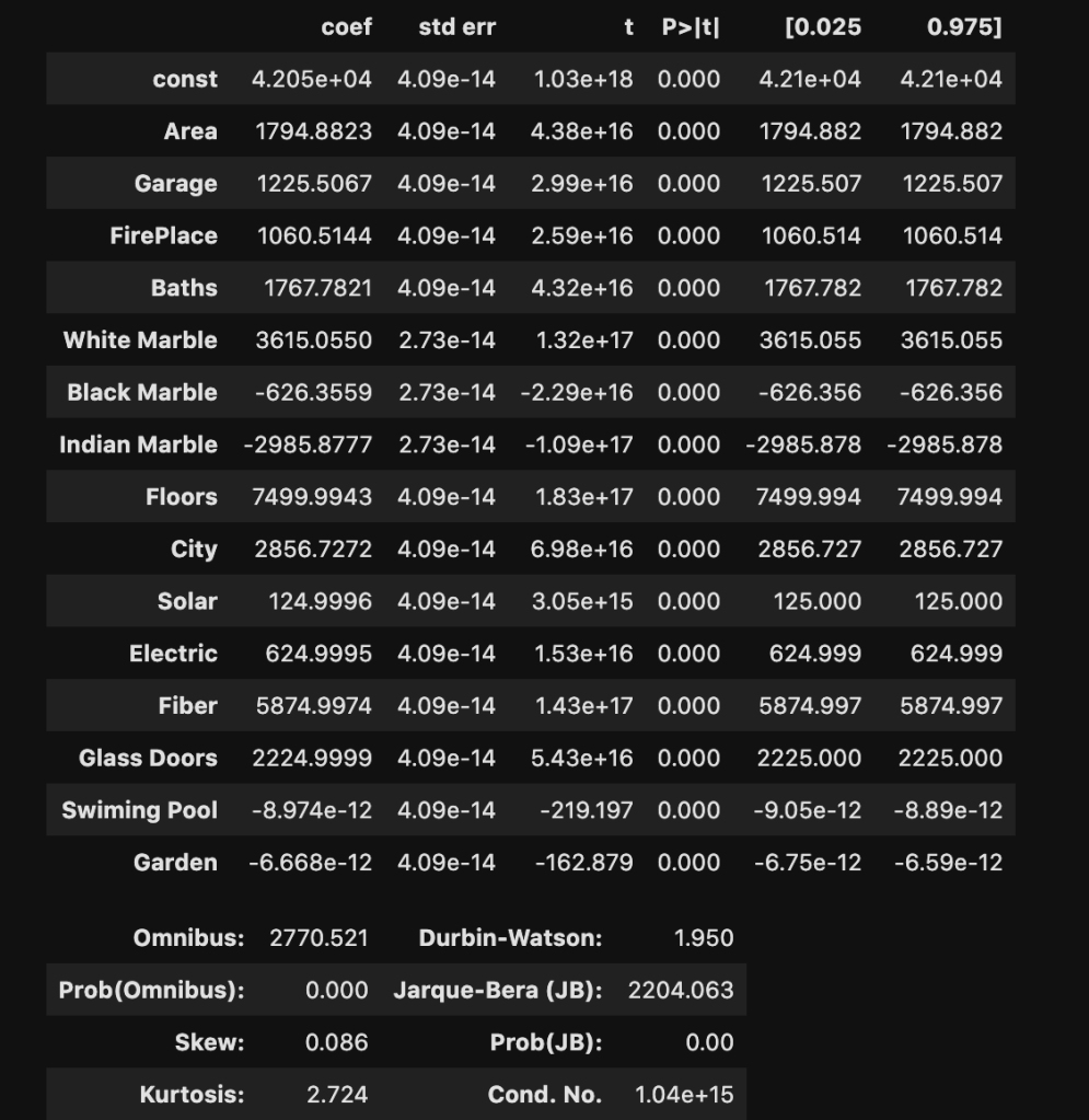
I won’t bore you with details that much. Just notice how much we were able to extract and understand in a simple three lines of code. If you’re confused, here is what you should know: R-squared is a scale of 0 to 1 representing how good your model is. 1 is the best score. Also the coef column, which we will look at later, represents coefficients. (The coefficients here make me really skeptical that this is real data. Although, that view comes from a Chicagoan’s perspective. I’m sure the dynamic changes as you move around geographically, though).

Sklearn Method

This is the method I use most often. In the code below, I create, train, and validate a regression model.

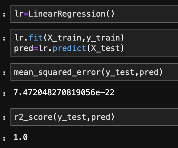
In terms of coefficients:

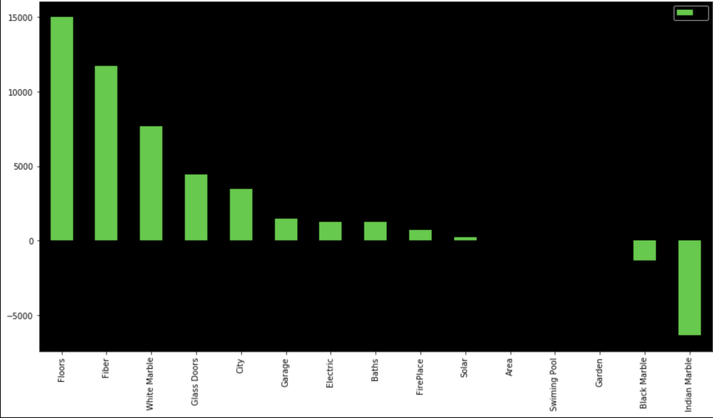
Even though regression can get fairly complex, running a regression is pretty simple once the data is ready. It’s also a nice data set as my R-squared is basically 100%. That’s obviously not realistic, but that’s not the point of this blog.

Conclusion

While linear regression is a powerful and complex analytical process, it turns out that running regression in the context of python, or other coding language, I would imagine, is actually quite simple. Checking assumptions is rather easy and so is creating, training, and evaluating models. That said, regression can get more difficult, but for less complex questions and data sets, it’s a fairly straight-forward process. So even if you have no idea how regression really works, you can fake it to some degree. In all seriousness, though, you can draw meaningful insights, in some cases, with a limited background.

Thanks for reading!

Further Reading

(https://towardsdatascience.com/assumptions-of-linear-regression-5d87c347140)