Acquiring a baseline understanding of the ideas and concepts that drive linear regression.

Introduction

Thanks for visiting my blog!

Today, I’d like to do my first part in a multi-part blog series discussing linear regression. In part 1, I will go through the basic ideas and concepts that describe what a linear regression is at its core, how you create one and optimize its effectiveness, what it may be used for, and why it matters. In part 2, I will go through a concept called gradient descent and show how I would build my own gradient descent, by hand, using python. In part 3, I will go through the basic process of running linear regression using scikit-learn in python.

This may not be the most formal or by-the-book guide, but the goal here is to build a solid foundation and understanding of how to perform a linear regression and what the main concepts are.

Motivating Question

Say we have the following (first 15 of 250) rows of data (it was randomly generated and does not intentionally represent any real world scenario or data):

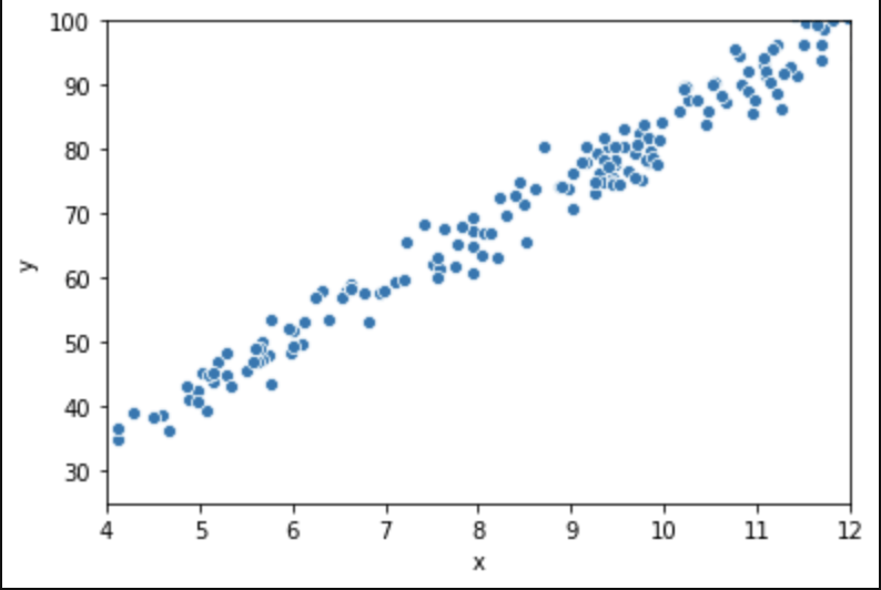
Graphically, here is what these 250 rows sort of look like:

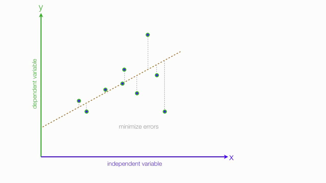
We want to impose a line that will guide our future predictions:

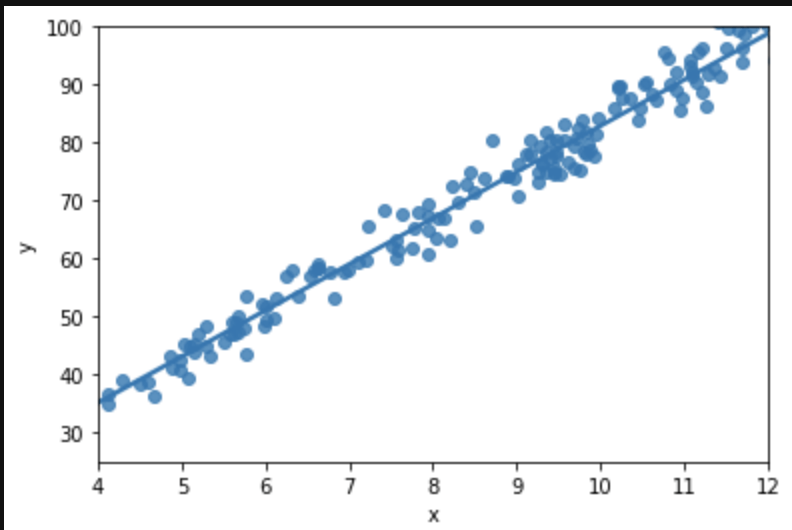
The above graph displays the relationship between input and output using a line, called the regression line, that has a particular slope as well as a starting point, the intercept, which is an initial value added to each output and in this case sits around 35. Now, if we see the value 9 in the future as an input, we can assume the output would lie somewhere around 75. Note that this closely resembles our actual data where we see the (9.17, 77.89) pairing. Moving on, this corresponds on our regression line to an intercept of 35 + 9 scaled by the slope which might be around 40/9, or 4.5. Or in basic algebra y=mx+b: 75 = 4.5*9 +35. That’s all regression is! Basic algebra using scatter plots. That was really easy I think. Now keep in mind that we only have one input here. In a more conventional regression, we have many variables and each one has its own “slope,” or in other words, effect on output. We need to use more complex math to allow for the ability to measure the effect of every input. For this blog we will consider the single input case, though. It will allow us to have a discussion about how linear regression works as a concept and also give us a starting point to think about how we might change our approach, or really adjust our approach, as we move into data that is contextualized or described in 3 or more dimensions. Basic case: find effect of height on wingspan. Less basic case: find effect of height, weight, country, and birth year on life expectancy. Case 2 is far more complex but we will be able to address it by the end of the blog!

Assumptions

Not every data set is suited for linear regression; there are rules, or assumptions, that must be in place.

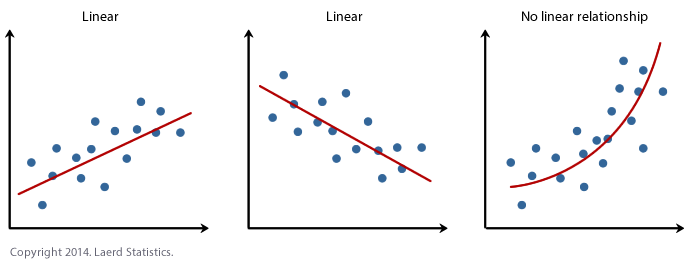
Assumption 1: Linearity. This one is probably one you already expected, just didn’t know you expected it. We can only use LINEAR regression if the relationship shown in the data is, you know, linear. If the trend in the scatter plot looks like it needs to be described using some higher degree polynomial or other type of non-linear function like a square root or logarithm than you probably can’t use linear regression. That being said, linear regression is only one method of supervised machine learning for predicting continuous outputs. There are many more options. Let’s use some visuals:

Now, you may be wondering the following: this is pretty simple in the 2D case, but is it easy to test this assumption in higher dimensions? The answer is yes.

Assumption 2: Low Correlation Between Predictive Features. Our 2D case is an exception in a sense. We are only discussing the simple y=mx+b case here and the particular assumption listed above is more suited to multiple linear regression. Multiple linear regression is more like y= m1x1+m2x2+…+b. Basically, it has multiple independent variables. Say you are trying to predict how many points a game a player might score on any given night in the NBA and your features include things like height, weight, position, all-star games made, and some stats about how their vertical leap or running speed. Now, let’s say you also have the features that say a player’s age and what year they were drafted. Age and draft year are inherently correlated. We would probably not want to use both draft year and age. We know what this idea of reducing correlation means by using that example, but why is it important to reduce correlation? Well, one topic to understand is coefficients. Coefficients are basically the conclusion of a regression. They tell us how important each feature is and what its impact is on output. In the y=mx+b equation, m is the coefficient of x, the independent variable, and basically tells us how the dependent variable responds to each x value. So if you have an m value of 2 it means that the output variable increases by twice the value of the input variable. Say you are trying to predict NBA salary based on points per game. Well, let’s use two data points. Stephen Curry makes about $1.5M per point averaged and LeBron James makes about $1.4M per point averaged. Now, these players are outliers, but we get a basic idea that star players make like $1.45M per point averaged. That’s the point of regression; finding causal relationship between input and output. We lose the ability to find the impact of unique features on output when there are highly correlated features as they often move together and represent being tied together in certain ways.

Assumption 3: Homoscedasticity. Basically, what homoscedasticity means is that there is no “trend” in your data. What do I mean by “trend?”. By this, I mean that if you take a look at all the error values in your data (say your first value is 86 and you predict 87 and the second prediction is 88 but the true value is 89, then your first two errors are valued at 1 and -1), whether positive or negative, and plot it around the line y=0 representing no error, then we would not see a pattern in the resulting scatter plot and we might assume that the points around that line (y=0) would look to be rather random and most importantly, have constant variance. This plot we just described, that has a baseline of y=0 and error terms around it is called a residual plot. Let me give you the visual you have been waiting for in terms of residual plots. Also note that we didn’t discuss heteroscedasticity – but it’s basically the opposite of homoscedasticity, I think that’s quite obvious.

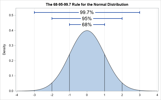
Assumption 4: Normality. This means that distribution of the error of the points that fall above and below the line is normally distributed. Note that this refers to the distribution of the value of the error (also called residuals – the value of which is calculated by subtracting the true value from the estimated value at every single value in the scatter plot measured against the closest value in the regression line), not the distribution of the y values. Here is a basic normal distribution. Hopefully, the largest portion of the value of the residuals fall around a center point (not necessarily at the value zero, it’s just an indicator of zero standard deviations from the mean – that’s what the x-axis is) and the amount of smaller and larger residuals appear in smaller quantities.

This next graph shows where the residuals should fall to have normality present, with E(y) representing the expected value (Credit to Brandon Foltz from YouTube for this visual).

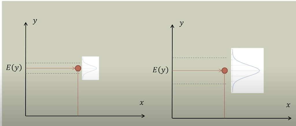
Both graphs work, but at different scales.

Fitting A Line

Ok, so now that we have our key assumptions in place, we can start searching for the line that best fits the data. The particular method I’d like to discuss here is called ordinary least squares, or OLS. OLS sums up the difference between every predicted point and every true value (once again, each of those values is called a “residual,” which represents error) and squares this difference, adds it to the sum of residuals, and divides that final sum over the total number of data points. We call this metric MSE; mean squared error. So it’s basically finding the average error and looking for the model with lowest average error. To do this, we optimize the slope and intercept for the regression line so that each point is as close as possible to the true value as judged by MSE. As you can see by the GIF below, we start with a simple assumptions and move quickly toward the best line but slow down as we get closer and closer. (Also notice that we almost always start with assumption of a slope of zero. This is basically testing the hypothesis that input has no effect on output. In higher dimension, we always start with the simple assumption that every feature in our model has no effect on output and move closer to its true value carefully. This idea relates to a concept called gradient descent which will be discussed in the next blog in this series).

Now, one word you may notice that I used in the paragraph above is “optimize.” In case, you don’t already see where I’m going with this, we are going to need calculus. The following equation represents error and the metric we want to minimize as discussed above.

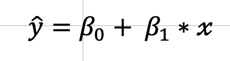
That E looking letter is the Greek letter Sigma which represents a sum. The plain y is the true value (one exists for every value of x), and the y with a ^ (called y-hat) on top represents the predicted value. We basically square these terms so that we can look at error in absolute value terms. I would add a subscript of a little “n” next to every y and y-hat value to indicate that there are like a lot of these observations. Now keep in mind, this is going to be somewhat annoying to derive, but once we know what our metrics are we can use the formulas going forward. To start, we are going to expand the equation for a regression line and write it in a more formal way:

So, now we can look at MSE as follows:

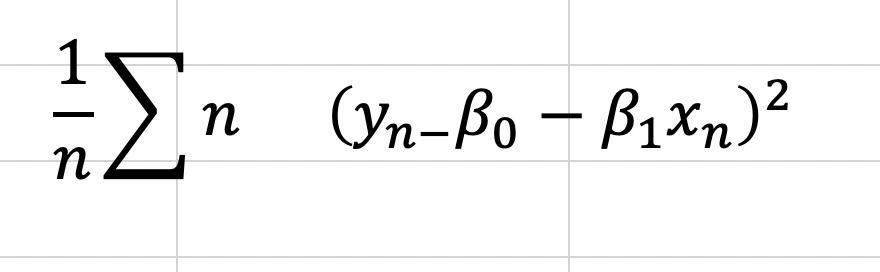
This is the equation we need to optimize. To do this we will take the derivative with respect to all of our two unknown constants and set those results equal to zero. I’m going to do this by hand and add some pictures as typing it would take a while.

Step 1: Write down what needs to be written down; the basic formula, a formula where I rename the variables, and the partial derivatives for each unknown (If you don’t know what a partial derivative is that’s okay, it just tells us the equation we need to set equal to zero, because at zero we have a minimum in the value we are investigating, which is error in this case. Both error for slope value and error for intercept value. Those funky swirls that with the letters F on top and A or B below represent those equations).

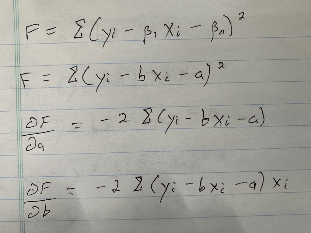
Conclusion: We have everything we need to go forward.

Step 2: Solve one equation. We have two variables, and in case you don’t know how this works, we will therefore need two equations. Let’s start with the simpler equation.

Conclusion: A, or our intercept term equals the average of y, as indicated by the bar, minus the slope scaled by the average of x (keep in mind this is an average due to the 1/n, or “1 over N”, term not included. Also remember that for the end of the next calculation).

Step 3: Solve the other equation, using substitution (apologies for the rotation).

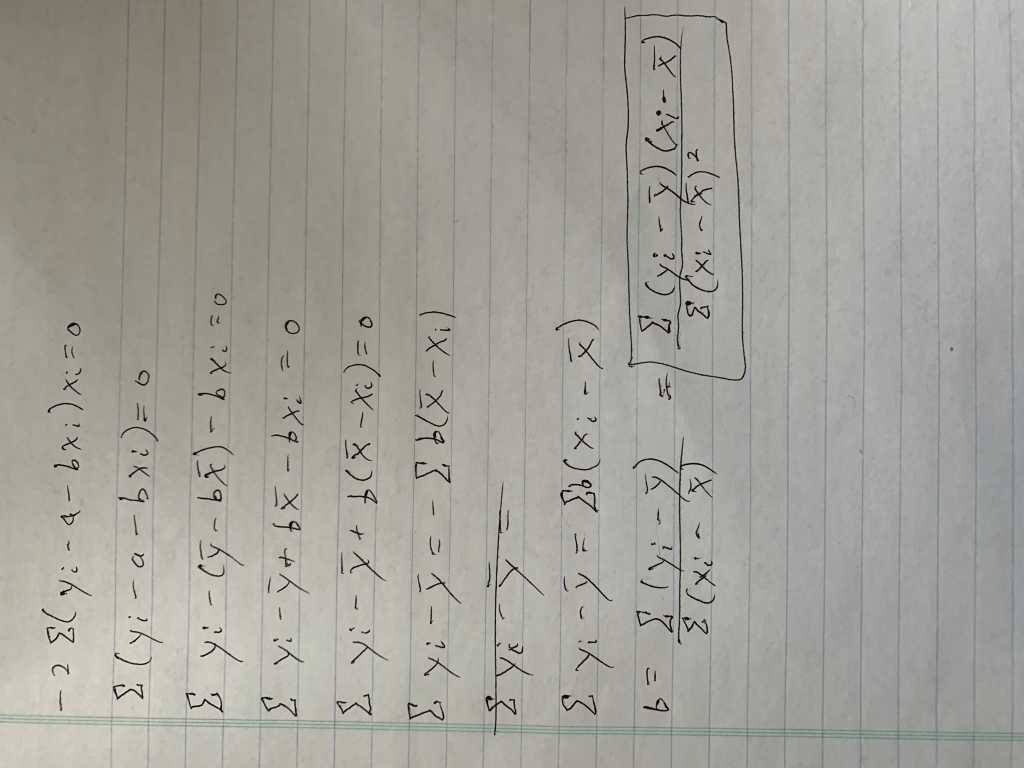
Conclusion: After a lot of math we got our answer. You may notice I took an extra step at the end and added a little box around that extra step. The reason for this is because that equation (hopefully, at the very least, you have encountered the denominator before) in that box is equal to the covariance between x and y divided by the variance of x. Those equations are fairly simple but are nevertheless beyond the scope of this blog. Let’s review how we calculate slope.

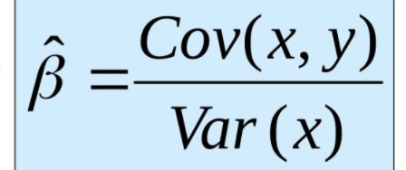
That was annoying, but we have our two metrics! Keep in mind that this process can be extended with increased complexity to higher dimensions. However, for those problems, which will be discussed in part 3, we are just going to use python and all its associated magic.

Evaluating Your Model

Now that we know how to build a basic slope-intercept model, how can we evaluate whether or not it is effective? Keep in mind that magnitude of the data you model may change which means that looking at MSE and only MSE will not be enough. We need the MSE to know what to optimize for low error, but we are going to need a bit more than that to evaluate a regression. Let’s now discuss R-Squared. R-Squared is a 0-1 or 0%-100% scale of how much variance is captured by our model. That sounds a bit weird and that’s because it’s a rather technical definition. R-Squared really answers the following question: How good is your model? Well, 0% means your model is the worst thing since the New York Yankees were introduced. A score in the 70%-90% range is more desirable. (100%, which you are no doubt wondering why I didn’t pick, means you probably overfit on training data and made a bad model). This is all nice, but how do we calculate this metric?

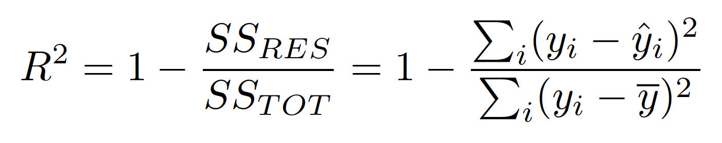
One minus the sum of each prediction’s deviation from the true value divided each true value’s deviation from the mean (with both the numerator and denominator squared to account for that absolute value issue discussed earlier). You can probably guess the SS-RES label alludes to the concept of residuals and the sum of squares from residuals; true values minus the predicted values squared. The bottom refers to total sum of squares; a metric for deviation from the mean. In other words, (one minus) the amount of error in our model versus the amount of total error. There is also metric you may have heard of called “Adjusted R-Squared.” The idea behind this is to penalize excessively complex models. We are looking at a simple case here with only one true input, so it doesn’t really apply. Just know it exists for other models. Keep in mind that R-Squared doesn’t always measure how effective you in particular were at creating a model. It could be that it’s just a hard model to construct or one that will never work well independent of who creates the model. (Now you may be wondering how to people can have a different regression model. It’s a simple question but I think it’s important. The real difference between two models can present themselves in many ways. A key one, for example, is how one decides to pre-process their data. One person may remove outliers to different degrees than others and that can make a huge difference. Nevertheless, even though models are not all created equally, some have a lower celling or higher floor than others for R-Squared values).

Conclusion

I think if there’s one point to take home from this blog, it’s that linear regression is a relatively easy concept to wrap your head around. It’s very encouraging that such a basic concept is also highly valued as a skill to have as linear regression can be used to model many real world scenarios and has so many applications (like modeling professional athlete salaries or forecasting sales). Linear regression is also incredibly powerful because it can measure the effect of multiple inputs and their isolated impact on a singular output.

Let’s review. In this blog, we started by introducing a scenario to motivate interest in linear regression, discussed when it would be appropriate to conduct linear regression, broke down a regression equation into its core components, derived a formula for those components, and introduced metrics to evaluate the effectiveness of our model.

From my perspective, this blog presented me with a great opportunity to brush up on my skills in linear regression. I conduct linear regression models quite often (and we’ll see how those work in part 3) but don’t always spend a lot of time thinking about the underlying math and concepts, so writing this blog was quite enjoyable. I hope you enjoyed reading part 1 of this blog and will stick around for the next segment in this series. The next concept (in part 2, that is) I will discuss is a lesser known concept (compared to linear regression) called gradient descent. Stay tuned!

Sources and Further Reading

(https://warwick.ac.uk/fac/soc/economics/staff/vetroeger/teaching/po906_week567.pdf)

(http://www.mit.edu/~6.s085/notes/lecture3.pdf)

(https://medium.com/next-gen-machine-learning/r-square-coefficient-of-determination-f4f3c23329d9)

(https://medium.com/analytics-vidhya/r-squared-vs-adjusted-r-squared-a3ebc565677b)

(https://medium.com/@rahul77349/what-is-multicollinearity-5419c81e003f)

(https://towardsdatascience.com/linear-regression-for-data-science-1923256aba07)

(https://towardsdatascience.com/assumptions-of-linear-regression-algorithm-ed9ea32224e1)